(1.1)
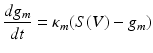
Where V represents the membrane potential, C represents the membrane capacitance, g m —the conductance of a particular ion-channel, V m is this ion’s reversal potential and I(t) represents the external input to the cell. Then conductance states—describing the state of an active ion channel can also be given appropriate dynamic constraints based on receptor time constants and the number of open channels at that cell:
(1.2)
Where S can represent a sigmoidal activation function describing population firing averages or can be replaced with a Heaviside function to mimic the all-or-nothing properties of single cell firing—both dependent on the afferent’s cell membrane depolarization V. Different ionic currents can be incorporated when modelling different brain regions—for example in Chap. 4 these type of currents are used to describe connected networks of the thalamus and basal ganglia where currents through the Globus Pallidus differ from those exciting thalamus, in accordance with known neurophysiology.
Neural Field Models
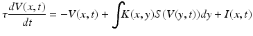
These types of formulations do not include a description of the spatial characteristics of cell activity. For this reason, some authors employ partial differential equations in what are called in this book—neural field models. Hutt and colleagues in Chap. 6 introduce a simple example of this—the so-called Amari model—whereby synaptic temporal dynamics are augmented with a spatial kernel representing a d-dimensional cortical manifold;
(1.3)
Here, the membrane potential is described in both space x, and time t—and can accommodate the same type of applied inputs I(x, t) as above, while also allowing for spatially distributed inputs through kernel K. Simplifications, such as spatial homogeneity and isotropic input can be applied with a simple kernel function: K(x, y) = K(||x − y||), while more elaborate constraints, for example specific intralaminar profiles of connectivity can be incorporated into these neural field models as explicated in Marreiros and colleagues in the dynamic causal models for neural fields.
Validation Approaches
So what makes a good model? Famous lines of thought on this issue include George Box’s epigram—“Essentially, all models are wrong, but some are useful” [2], or Rosenblueth and Wiener’s—“The best material model of a cat is another, or preferably the same cat” [11]. This—of Rosenblueth and Wiener—is in fact the truncated (and more famous) version of their full writing which was preceded “That is, in a specific example, the best material model…”. This oft omitted qualifier highlights the delicate balance that must be achieved by models of neuronal processes that have adequate detail to describe the key features under study while also being able to generalize to other data sets and potentially to other disorders. This is a clear achievement of the authors of this book—who highlight the generalizability of their modeling approaches by illustrating different applications of the underlying biophysical fundaments to different brain regions and cell types, different control regimes and to multiple diseases or brain states.
In addition, the authors develop their own internal validation criteria. In Chap. 5, Robinson and colleagues outline particular criteria that should be met when developing and applying biophysical models of neuronal dynamics. These include (1) that the model be based on anatomy and physiology and incorporate different spatial and temporal scales, (2) that they provide quantitative predictions that can be experimentally corroborated, (3) that parameters of the model can be constrained through independent manipulations of the brain, (4) that they generalize to multiple brain states and (5) that they be invertible. While the models applied in the chapters that precede and follow Robinson et al. all conform to criteria 1–4 only certain authors discuss and implement model invertibility; criteria 5. However model invertibility may serve as a useful criterion for measuring model goodness and grandfather other criteria for a number of reasons. Firstly an invertible model is a model where parameter values can be recovered from simulated or empirical data—hence it directly assesses model complexity and generalizability. If the model is too simple then empirical data from a variety of sources should reveal features of the data that are not adequately captured by the model—and in the other direction—if the model is too complex then simulated changes in parameter values will not be recovered in a multi-start inversion scheme since parameter redundancy should be revealed by changes in “the wrong” parameter.
This fifth criterion is explicitly addressed by Dynamic Causal Models (Chap. 3). This model framework uses a variational Bayesian inversion scheme to recover the underlying parameter space from real and simulated data. In this context, we learn in Chap. 3 that DCMs are subject to three forms of validation, namely tests of (1) face validity, (2) construct validity and (3) predictive validity. The first here, face validity is a test of model invertibility. DCMs specify the dynamics of layered neuronal ensembles comprising interconnected with distinct cell types and ion channels with parameters that encode, for example, synaptic connectivity and receptor time constants. By simulating across regions of parameter space and applying the inversion routine, the repertoire of these models are revealed—e.g. different spectra as well as the goodness of parameterization. Formally the inversion procedure produces a metric of model-goodness known as the negative Free Energy, which is an approximation to the model evidence and allows competing models or hypotheses to be tested. This metric is similar to the Akaike Information Criterion or the Bayesian Information criterion but can incorporate a priori parameter values and co-dependencies among parameters. Construct validity is the test of whether estimates of parameter values reflect the underlying biological reality. This is linked to Robinson’s criterion 4– where alterations in parameters of the model that lead to changes in model output should be testable using some independent manipulation of the brain component that that parameter is thought to represent.
Throughout the book we see examples of this construct validity using pharmacological manipulations as independent verification. For example in Chap. 2, Érdi and colleagues report that zolpidem—a benzodiazepine that agonizes inhibitory GABAA receptors has been independently shown to alter (decrease) the frequency of theta frequency in hippocampal circuits—a finding they uncovered using their model in a comparison of AMPA vs. GABA receptor parameter function. Similarly in Chap. 6, Hutt and colleagues describe how neural field models recapitulate empirical EEG spectra under general anaesthesia by increasing their models GABAA receptor time constant. In Chap. 9 Coyle and colleagues present a similar validation; recapitulating key features of EEG spectra in Alzheimer’s disease.
Face validity is a vital first step in proposing a de novo model and is explored deeply in Chap. 10 by Herald and colleagues. They take on a very high-dimensional challenge—to uncover networks from spikes. Their ambitious and remarkable work is keenly motivated by the sampling problem—how can a systematic causality be ascribed to spiking neurons in samples where only “a handful” of spikes can be distinguished from a cultures containing as many as ten thousand members? Their results are highly promising—using a “shift set” metric they build measures of pair-wise causality and choose careful surrogate techniques to illustrate the ability to sample above stochastic process noise. Useful for researchers in this wide field is their provision of a temporal limit on the length of time a recording will render useful pairwise statistics—it’s about 850 msec.
Predictive validity is potentially the most useful but the least tested aspect of model validation in this book—indicative of a still maturing field. In this book the authors describe particular features of predictive validity both in terms of prior and future work. Predictive validity refers explicitly to the application of a model—what have you designed it to do? In essence, it is the final test of a model, where that model generates a quantitative measurement that is unknown after model inversion or simulation, but will be revealed as correct or incorrect after some additional empirical data have been acquired. (Table 1.1)
Table 1.1
A summary of model validation criteria addressed


