(1)
Cognitive Function Clinic, Walton Centre for Neurology and Neurosurgery, Liverpool, UK
Abstract
This chapter examines the methodology used to assess the diagnostic accuracy of clinical signs, cognitive and non-cognitive screening instruments used in the cognitive disorders clinic to assist in the diagnosis of dementia. The relevance of pragmatic diagnostic accuracy studies, compared to experimental studies, as a better reflection of the idiom of clinical practice, is emphasized.
Keywords
DementiaDiagnosisDiagnostic accuracy studiesDiagnostic criteria2.1 Methodology
A standardised methodology for the pragmatic study of the diagnostic utility of neurological signs, cognitive, and non-cognitive screening instruments has been used in the Cognitive Function Clinic (CFC; see Chaps. 3, 4 and 5 respectively).
Generally, consecutive new patient referrals have been examined for the sign or administered the test instrument being studied. Hence, in accordance with the idiom of clinical practice, a passive case finding strategy has been pursued (as in other long-term studies, e.g. Larner 2011a, b). In consequence, these are pragmatic or observational studies, as contrasted with index or experimental studies which are often undertaken to examine the diagnostic accuracy of tests. Clearly both approaches involve selection bias, and the particular paradigm chosen will depend, at least in part, on which type of selection bias is deemed preferable or least objectionable.
Clinical assessment has been by means of semi-structured patient interview, collateral history (where available), with or without formal neuropsychological assessment (e.g. Wechsler Adult Intelligence Scale Revised, National Adult Reading Test, Wechsler Memory Scale III, Graded Naming Test, Rey-Osterrieth Complex Figure, Stroop colour-word test, verbal fluency tests), and structural neuroimaging (CT ± MRI; see Sect. 6.2.1). There has been only limited access to functional neuroimaging with HMPAO-SPECT (Doran et al. 2005) or 1H-magnetic resonance spectroscopy (Larner 2006a, 2008; Sect. 6.2.2), and to CSF biomarkers. Diagnosis has been based on clinician judgement, using widely accepted clinical diagnostic criteria (see Sect. 2.2).
The standard clinical paradigm is cross-sectional (i.e. interindividual) patient assessment, but cognitive disorders often require longitudinal (i.e. intraindividual) patient assessment in order to establish a diagnosis. Longitudinal use of some cognitive screening instruments has been undertaken (Larner 2006b, 2009a, b). Occasionally tests have been applied to non-consecutive patient cohorts, for example when a specific diagnostic question is being addressed, on the basis that tests are essentially used to provide arguments for a given diagnosis that is suspected by a clinical assessment (e.g. use of the Frontal Assessment Battery in patients whose differential diagnosis encompassed behavioural variant frontotemporal dementia, and Fluctuations Composite Scale in patients whose differential diagnosis encompassed a synucleinopathy; see Sects. 4.11 and 5.4.3 respectively). Clearly all clinic-based patient cohorts show selection bias in comparison to community-based samples, but nonetheless such samples still have a large clinical variability which will reduce test power.
The principles of evidence-based diagnosis have been followed (Qizilbash 2002) to calculate various parameters of diagnostic value based on a 2 × 2 data table (Fig. 2.1). Also sometimes known as a table of confusion or a confusion matrix, the 2 × 2 table shows binary test results cross-classified with the binary reference standard.
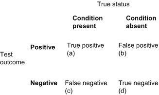

Figure 2.1
2 × 2 table (table of confusion, confusion matrix)
A large number of parameters may be calculated from the 2 × 2 table (see Box 2.1), of which only a few have been selected for routine use and to facilitate comparison between tests, viz. overall test accuracy (or correct classification accuracy), sensitivity (Se), specificity (Sp), Youden index (Y; Youden 1950), positive and negative predictive values (PPV, NPV), predictive summary index (PSI; Youden 1950), positive and negative likelihood ratios (LR+, LR−; Black and Armstrong 1986; Jaeschke et al. 1994; Deeks and Altman 2004), diagnostic odds ratios (DOR; Glas et al. 2003), positive and negative clinical utility index (CUI+, CUI−; Mitchell 2008, 2011; Mitchell et al. 2009), and area under the receiver operating characteristic (AUC ROC) curve (Lusted 1968; Hanley and McNeil 1982, 1983; Zweig and Campbell 1993). Whereas some authors cite the sum of sensitivity and specificity (e.g. McCrea 2008), in this analysis the Youden index has been preferred. In all cases, 95 % confidence intervals (CI) have been calculated: for sensitivity, specificity, and positive and negative predictive values, using p ± 1.96√p(1 − p)/n (Bourke et al. 1985:62); for likelihood ratios and diagnostic odds ratio using the log method (Clopper and Pearson 1934; Altman et al. 2000:108–110).
Box 2.1: Some Measures of Test Utility Applicable to Diagnostic Studies (See Also Fig. 2.1; Adapted from Larner 2013)
Overall test accuracy (Acc):


Sensitivity (Se): a measure of the correct identification of true positives:


Specificity (Sp): a measure of the correct identification of true negatives:


Youden index (Y), or Youden J statistic:


Positive predictive value (PPV): a measure of the probability of disease in a patient with a positive test, or the proportion of individuals that do possess a positive test who do have the diagnosis:


Negative predictive value (NPV): a measure of the probability of the absence of disease in a patient with a negative test, or the proportion of individuals that do not have a positive test who do not have diagnosis:


Predictive summary index (PSI):


False positive rate:


False negative rate:


False alarm rate:


False reassurance rate:


Positive likelihood ratio (LR+): odds of a positive test result in an affected individual relative to an unaffected individual, hence a measure of diagnostic gain, more readily applicable in the setting of an individual patient:


Negative likelihood ratio (LR−): odds of a negative test result in an affected individual relative to an unaffected individual, hence a measure of diagnostic gain, more readily applicable in the setting of an individual patient:
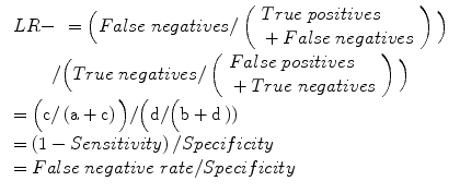

Diagnostic odds ratio (DOR):
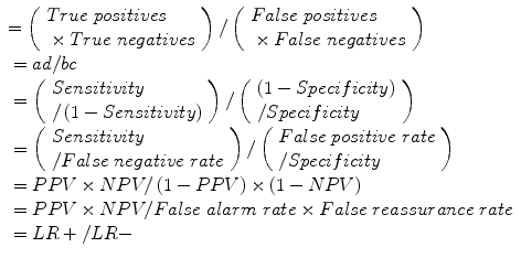

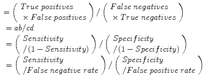
Error odds ratio (EOR):

Clinical utility index (CUI+, CUI−): calculates the value of a diagnostic method:


Receiver operating characteristic (ROC) curve: plot of false positive rate (1 – Specificity) on the x axis (abscissa) against sensitivity (“hit rate”) on the y axis (ordinate); area under the curve (AUC) is a measure of test diagnostic accuracy, where AUC = 0.5 indicates that a test provides no added information, and AUC = 1 indicates a test providing perfect discrimination.
Tables summarising metrological properties have been provided for each sign or test examined, using the cutoff (also sometimes known as threshold or dichotomisation point) which gave optimal overall test accuracy (usually for dementia/no dementia, but sometimes for any cognitive impairment/no cognitive impairment): this may differ from the cutoff quoted in index (experimental) studies. Different test cutoffs might of course be applied in practice to maximise either sensitivity (at the cost of lower specificity) or specificity (at the cost of lower sensitivity), as per clinician requirements. It is also important to remember in this context that numbers are not diagnoses: administering any screening instrument is part of the clinical assessment and includes a qualitative judgement on the part of the clinician which may inform diagnostic considerations.
Because patients may sometimes not be tested with either the index test or reference standard, some authors advocate the use of an “intention to diagnose” approach (analogous to intention to treat in clinical therapeutic trials) with a 2 × 3 table rather than the standard 2 × 2 table (Schuetz et al. 2012). Because most patients seen in CFC have been testable, this approach has not been used, but note has been made when and why occasional patients have not been tested.
Statistical methods have been described as the “technology of handling uncertainty” (Hand 2008:2,55). Simple statistical methods amenable to pen, paper and pocket calculator have been used (e.g. Swinscow 1983; Bourke et al. 1985; Altman et al. 2000) in these studies (i.e. datasets have been handled manually; suitable calculators for these parameters also exist, e.g. www.psycho-oncology.info/Clinical_utility_index_calculator_ajmitchell2012.xls). The Standards for the Reporting of Diagnostic accuracy studies (STARD) checklist has been observed (Bossuyt et al. 2003a, b). The studies reported predate the publication of the STARDdem guidelines, i.e. STARD guidelines specific to diagnostic accuracy studies in dementia (www.starddem.org).
Sample size calculations have not been performed, as is sometimes recommended for diagnostic accuracy studies (Bachmann et al. 2006). A pragmatic approach to sample size estimates has suggested that normative ranges for sample sizes may be calculated for common research designs, with anything in the range of 25–400 being acceptable (Norman et al. 2012).
For the calculation of p values, a value of p < 0.05 has been deemed significant. For categorical nonparametric analyses, χ2 test has been used.
Regarding the diagnostic value of these various tests, parameters previously recommended for ideal biomarkers of Alzheimer’s disease by The Ronald and Nancy Reagan Research Institute of the Alzheimer’s Association and the National Institute on Aging Working Group (1998) have been deemed appropriate and desirable, namely sensitivity and specificity no less than 80 % and PPV approaching 90 %. PPV and NPV are measures, respectively, of the probability of disease in a patient with a positive test, and of the absence of disease in a patient with a negative test; these parameters are influenced by the prevalence of the disease in the population being tested. Some authors have argued for the paramount importance of PPV rather than sensitivity for neuropsychological measures (Smith and Bondi 2013:19–20).
Likelihood ratios measure the change in pre-test to post-test odds, and hence are measures of diagnostic gain. They are particularly useful in clinical practice since they are more readily applicable to an individual patient than sensitivity and specificity; moreover, their calculation does not depend on prevalence rates. LR+ is the odds of a positive test result in an affected individual relative to an unaffected individual; LR− is the odds of a negative test result in an affected individual relative to an unaffected individual (Deeks and Altman 2004). LRs can vary dramatically between different populations, and cannot be used in differential diagnostic reasoning (Llewelyn 2012). Likelihood ratio values range from 1–∞ (LR+) and 0–1 (LR−), and may be classified as large, moderate, small, or unimportant (Box 2.2).
Box 2.2: Classification of Likelihood Ratios
Large | Moderate | Small | Unimportant | |
|---|---|---|---|---|
LR+ | >10 | 5–10 | 2–5 | 1–2 |
LR− | <0.1 | 0.1–0.2 | 0.2–0.5 | 0.5–1 |
Diagnostic odds ratio (DOR) is desirably as large as possible; if either cell b or c in the 2 × 2 table (False positive or False negative) is zero then DOR is infinite, denoted by a lemniscate (∞).
For the clinical utility index (CUI+, CUI−), values range from 0 to 1, and performance may be classified as excellent, good, adequate, poor, or very poor (Box 2.3):
Box 2.3: Classification of Clinical Utility Indexes (After Mitchell et al. 2009)
Stay updated, free articles. Join our Telegram channel

Full access? Get Clinical Tree


