Fig. 1.1
A bookcase containing three different objects (a marker, a rectangular-shaped object and a mug), placed at five different positions, at three different shelves, is depicted. A superimposed diagram presents the distances between the different object positions. These five positions were used for both types of experiments
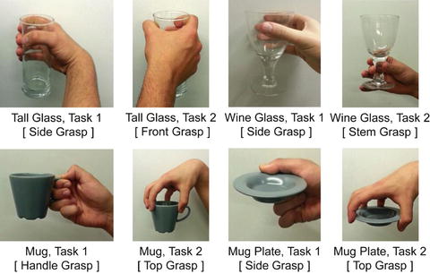
Fig. 1.2
Tasks executed for the second type of experiments. The tall glass tasks were: task 1, side grasp (to drink from it) and task 2, front grasp (to transpose it). The wine glass tasks were: task 1, side grasp (to drink from it) and task 2, stem grasp (to drink from it). The mug tasks were: task 1, handle grasp (to drink from it) and task 2, top grasp (to transpose it). Finally the mug plate tasks were: task 1, side grasp (to lift and hold it) and task 2, top grasp (to transpose it)
The first type of experiments, involved reach to grasp movements towards different positions (five different positions depicted in Fig. 1.1) and different objects (a mug, a rectangular shaped object and a marker) and was used for EMG-based “subspace discrimination” and “object discrimination”. The second type of experiments, involved reach to grasp movements towards specific positions and objects, in order to execute two different tasks (two classes), with the same object. A tall glass, a wine glass, a mug and a mug plate were used for the second type of task discrimination experiments. The first experiments were used for the initial formulation of the learning framework proposed in [34] and were once again used in [38] together with the second type of experiments, to discriminate between different tasks and compute feature variables importance for different positions, objects and tasks.
The tasks executed for the second type of experiments appear in Fig. 1.2. During the experiments, each subject conducted several trials, for each position, object and task combination. In order to ensure data quality and avoid fatigue, adequate resting time of 1 min, was used between consecutive trials.
1.2.2 Motion Data Acquisition
In order to capture efficiently human kinematics – using appropriate motion capture systems – the kinematic models of the human arm and the human hand must be described. The kinematic model of the human arm, that we use in this study, consists of three rotational degrees of freedom (DoFs) to model shoulder joint, one rotational DoF for elbow joint, one rotational DoF for pronation-supination and two rotational DoFs for wrist flexion/extension and abduction/adduction. The kinematic model of the human hand consists of 20 rotational DoFs, 4 for each one of the 5 fingers. Regarding fingers we used for the four kinematically identical fingers (index, middle, ring and pinky) three rotational DoFs to model flexion-extension of the different joints and one rotational DoF for abduction-adduction. Human thumb is modeled, using two rotational DoFs for flexion-extension, one rotational DoF for abduction-adduction and one rotational DoF to describe palm’s mobility that allows thumb to oppose to other fingers. The kinematic models of the human arm and hand are presented in Fig. 1.3.
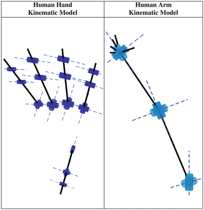
Fig. 1.3
Kinematic models depicting the degrees of freedom (DoFs) of the human arm and hand
In order to capture the human arm hand system motion in 3D space, extracting the corresponding joint angles (27 modeled DoFs), we used a dataglove for the human hand and a magnetic position tracking system for the human arm. The Isotrak II® (Polhemus Inc.) magnetic motion capture system used, is equipped with two position tracking sensors and a reference system. The two sensors of Isotrak II, were placed on the elbow and the wrist respectively, while the reference system was placed on the user’s shoulder. Having captured the positions of the human shoulder, elbow and wrist, the inverse kinematics of the human arm can be computed, following the directions provided in [39]. Alternatively for human robot interaction applications, a human to robot motion mapping procedure like the one proposed in [40], can be used. Regarding the human hand, the Cyberglove II® (Cyberglove Systems), is used to measure the 2 DoFs of the wrist (flexion-extension and abduction-adduction) and the 20 DoFs of the human fingers. The experimental setup that was used to track human arm hand system kinematics, is depicted in Fig. 1.4 and the different motion capture systems are depicted in Fig. 1.5.
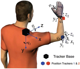
Fig. 1.4
Two position tracking sensors of Isotrak II are used to capture user’s shoulder, elbow and wrist position in 3D space, while a dataglove is used to capture the wrist and fingers joint angles. The position tracker reference system is placed on the shoulder. The human arm joint values can be computed through the human arm’s inverse kinematics. q 1 and q 2 jointly correspond to shoulder flexion-extension and adduction-abduction, q 3 to shoulder internal-external rotation, q 4 to elbow flexion-extension, q 5 to pronation-supination and q 6 and q 7 jointly correspond to wrist flexion-extension and adduction-abduction
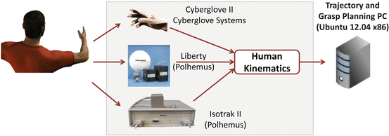
Fig. 1.5
Different motion capture systems, used to capture human arm hand system motion, are depicted
1.2.3 Electrode Positioning and EMG Data Acquisition
In total, we recorded the myoelectric activity of 16 muscles, of the upper arm (8 muscles) and the forearm (8 flexor and extensor muscles). More specifically the chosen muscles are: flexor pollicis longus, flexor digitorum superficialis, flexor carpi ulnaris, flexor carpi radialis, extensor pollicis longus, extensor indicis, extensor carpi ulnaris, extensor carpi radialis, deltoid anterior, deltoid posterior, deltoid middle, trapezius, teres major, brachioradialis, biceps brachii and triceps brachii. The selection of the muscles and the placement of the surface electromyography electrodes, was based on the related literature [16, 41]. In order to achieve easy, portable and fast to use training schemes several researchers have chosen to place the EMG electrodes, in specific regions but in random (not precise) positions [3]. We believe that the next generation of epidermal electronics [42] will make the electrode positioning faster and easier, thus we choose to take advantage of the higher signal to noise ratio, that accurate electrode positioning offers.
EMG signals were acquired and conditioned using an EMG system (Bagnoli-16®, Delsys Inc.), equipped with single differential surface EMG electrodes (DE-2.1®, Delsys Inc.). A signal acquisition board (NI-DAQ 6036E®, National Instruments), was used for signal digitization and data acquisition.
1.2.4 EMG and Motion Data Processing
Regarding data processing, EMG signals were band-pass filtered (20–450 Hz), sampled at 1 kHz, full-wave rectified and low-pass filtered (Butterworth, fourth order, 8 Hz), while for the position measurements, which were provided by the position tracking system at the frequency of 30 Hz, an antialiasing finite-impulse-response filter (low pass, order: 24, cutoff frequency: 100 Hz), was used to resample them at a frequency of 1 kHz (same as the sampling frequency of the EMG signals).
1.2.5 Muscular Co-activation Patterns Extraction
After data collection, all EMG recordings, were pre-processed and epochs of data were created. Those epochs included the different reach-to-grasp movements captured during the experiments. Then, all data were resampled at 100 Hz, where each sample at the new frequency (100 Hz) was calculated as the mean value of ten (10) samples of the original frequency (1 kHz). Based on the profiles of the rectified EMG signals at the new frequency, the onset of muscular activations was defined comparing the amplitude of each muscle’s myoelectric activation to it’s relaxed state. Finally, epochs including only muscular activations captured during the actual tasks were created, and were used to formulate synergistic profiles, using a novel statistical representation technique, that we introduced and which we call “Boxplot Zones”.
A boxplot (alt. box-and-whisker plot) is a method to graphically depict groups of numerical data, through the following five-number summaries: smallest observation (sample minimum), lower quartile (Q1), median (Q2), upper quartile (Q3), and largest observation (sample maximum). Boxplot zones were first defined in [34] to visualize muscular co-activation patterns and are an equivalent of boxplots, while more visually informative representation, suitable for the representation of synergistic profiles. Boxplot zones consist of three different layers. The first layer includes the median line, connecting the medians of all boxplots. The second layer includes the box zone (blue zone), connecting the boxes that contain all the values between the lower and the upper quartile, while the third layer includes the whisker zone (white zone), connecting the whiskers that mark the largest and the smallest observation. A direct comparison of a boxplot and a boxplot zone visualization, can be found in Fig. 1.6.
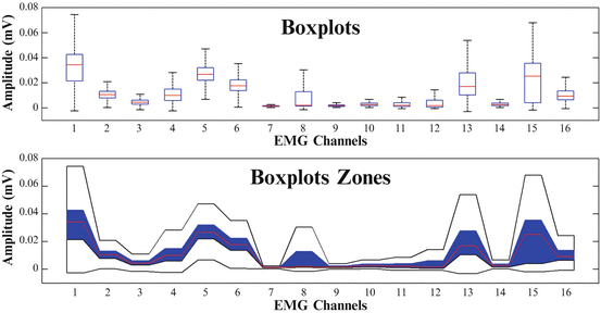
Fig. 1.6
Comparison of a Boxplot and a “Boxplot Zone” visualization of muscular co-activation patterns across sixteen (16) muscles of the upper arm and the forearm for one subject (Subject 1), performing reach to grasp movements towards a mug placed at position I
In Fig. 1.7 we present a “boxplot zones” based visualization of muscular co-activation patterns of sixteen (16) muscles (of the upper arm and the forearm), for one subject (Subject 1) executing reach to grasp movements, towards five (5) different positions in 3D space, to grasp three (3) different objects. The muscular co-activation patterns presented in Fig. 1.7 in terms of synergistic profiles formulated with boxplot zones, depict a significant differentiation between the different reach-to-grasp movements, although the same joints of the arm hand system (human upper arm joints and human hand finger joints) are involved, but for a different task. More precisely, if we examine the synergistic profiles (muscular co-activation patterns) across different subspaces (different positions), we notice that the activity of the muscles of the upper-arm (EMG channels 1–8) reflects most of the differentiation. In contrast, if we examine the muscular co-activation patterns across different objects, placed in the same subspace (a specific position), the activity of the muscles of the forearm (EMG channels 9–16) reflects most of the differentiation.
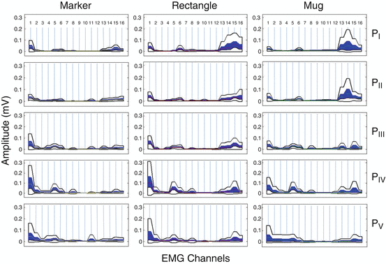
Fig. 1.7
“Boxplot Zones” visualization of muscular co-activation patterns of sixteen (16) muscles (of the upper arm and the forearm), for one subject (Subject 1) performing reach to grasp movements towards, five different positions (P I , P II , P III , P IV and P V ) in 3D space, to grasp three different objects (a marker, a rectangle and a mug). The sixteen (16) muscles are reported in the following order (1–16): deltoid anterior, deltoid middle, deltoid posterior, teres major, trapezius, biceps brachi, brachioradialis, triceps brachii, flexor pollicis longus, flexor digitorum superficialis, flexor carpi ulnaris, flexor carpi radialis, extensor pollicis longus, extensor indicis, extensor carpi ulnaris and extensor carpi radialis
In Fig. 1.8 we present a “boxplot-zones” based visualization of muscular co-activation patterns differentiation, for 16 muscles of the human upper-arm and forearm, for 3 different subjects performing different reach to grasp movements, towards five (5) different positions in 3D space, to grasp a specific object (rectangular-shaped object).
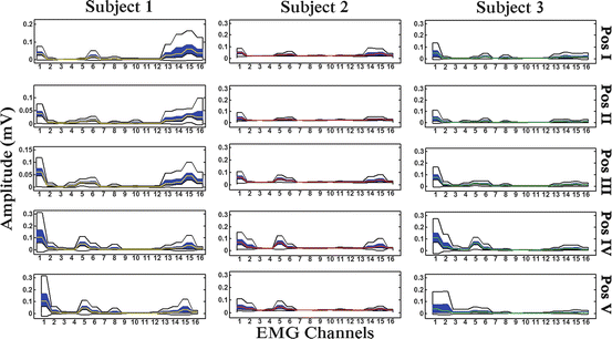
Fig. 1.8
“Boxplot Zones” visualization of different muscular co-activation patterns of sixteen (16) muscles of the upper arm and the forearm, for three (3) different subjects performing reach to grasp movements towards, the aforementioned five (5) positions in 3D space, to grasp a specific object (a rectangle)
As we have already noted there is a significant differentiation between muscular co-activation patterns associated with different reach to grasp movements. Statistical significance of muscular co-activation patterns differentiation, can be assessed using appropriate statistical tests. More precisely the Lilliefors test (adaptation of the Kolmogorov-Smirnov test) was used to test the null hypothesis that the EMG data – containing the myoelectric activations – come from a normal distribution. The test rejects the null hypothesis at the 5 % significance level (p = 0. 05), so the data are not normally distributed. Thus, we use non parametric tests such as, the Kruskal-Wallis and the Wilcoxon rank sum test, in order to assess the significance of muscular co-activation patterns differentiation, for different strategies.
The Kruskal-Wallis compares the medians of the myoelectric activity of the selected muscles, for different muscular co-activation patterns, and returns the p value for the null hypothesis that all samples are drawn, from the same population (or from different populations with the same distribution). The Wilcoxon rank sum test, performs a two-sided rank sum test of the null hypothesis that data of myoelectric activations with different muscular co-activation patterns, are independent samples from identical continuous distributions, with equal medians.
More details regarding the statistical procedures used, the reader can find in [43]. All tests were performed to check the differentiation of muscular co-activation patterns for the following three cases:
For the same reach to grasp movement, between different subjects.
For reach to grasp movements towards five different positions in 3D space.
For reach to grasp movements towards three different objects, placed at a specific position in 3D space.
For all sets, confidence levels were set at 95 %. All tests null hypotheses for all three cases were rejected, proving that muscular co-activation patterns differentiate, between different subjects and between different tasks. In Fig. 1.9, we present the means and the confidence intervals of EMG activity across eight muscles of the upper arm and eight muscles of the forearm, for a subject performing reach to grasp movements, towards three (3) different objects. In Fig. 1.10, we present the means and the confidence intervals of EMG activity across eight muscles of the upper arm and eight muscles of the forearm for a subject performing reach to grasp movements, towards a marker, placed at five (5) different positions in 3D space.
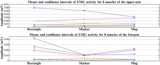
Fig. 1.9
Means and confidence intervals of EMG activity across eight (8) muscles of the upper arm and eight (8) flexor and extensor muscles of the forearm, for one subject (Subject 1) performing reach to grasp movements, towards three (3) different objects, placed at a specific position (Pos 3) in 3D space
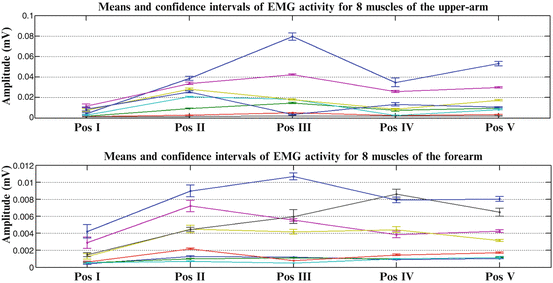
Fig. 1.10
Means and confidence intervals of EMG activity across eight (8) muscles of the upper arm and eight (8) flexor and extensor muscles of the forearm, for one subject (Subject 1) performing reach to grasp movements, towards a marker, placed at five (5) different positions in 3D space
Therefore, we conclude that the muscular co-activation patterns vary significantly not only between different subjects, but also between different reach-to-grasp movements of the same subject (towards different subspaces or different objects placed at specific position), and therefore should be considered and analyzed as subject-specific and task-specific characteristics.
1.3 Methods
In this section we present some typical specifications for EMG based interfaces and we describe the problem formulation and the methods used for discrimination of different muscular co-activation patterns, associated with different reach to grasp movements (classification) and EMG based motion estimation (regression).
1.3.1 Classification and Regression Modules
Some specifications that every EMG-based learning scheme should have, are:
To be able to “decide” on user’s intention (classification part).
To decode a continuous representation of human motion (regression part).
To allow its application at a robot control scheme, in real time.
To be easy and fast to be trained for different users (as musculoskeletal characteristics may vary significantly across subjects).
To be able to handle multidimensional spaces and large databases of myoelectric and motion data.
In this chapter we present an EMG-based learning scheme, using the Random Forests (RF) technique – which meets the aforementioned specifications – for both classification and regression. Thus, the classifier and the regressor cooperate advantageously, in order to split the task space and confront the non-linear relationship between the EMG signals the motion to be estimated, with task specific models that provide better estimation accuracy than the “general” models (built for all tasks).
In Fig. 1.11 we present a block diagram of a typical random forests based classification procedure. Random forests are used for a multiclass classification problem, where we need to discriminate between reach to grasp movements, towards different positions, different objects (to be grasped) and different tasks (to be executed with the object) in 3D space, using human myoelectric activity (EMG).
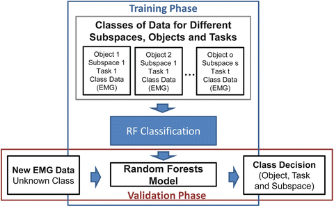
Fig. 1.11
Block diagram of the classification procedure
In Fig. 1.12 we present the block diagram for a typical random forests based regression procedure. The task specific models trained are used to estimate for new EMG data (not previously seen during training) “new” human arm hand system kinematics.
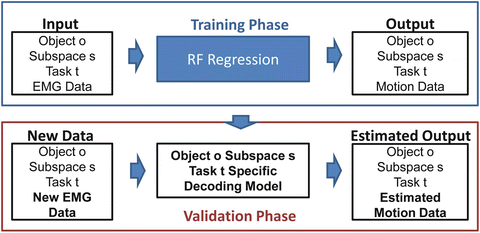
Fig. 1.12
Block diagram of the regression procedure
A complete block diagram of the EMG-based learning scheme proposed, is depicted in Fig. 1.13. Two main modules appear, the classification module and the task specific model selection module. Classification module provides decision for subspace to move towards, object to be grasped and task to be executed (with the object). Task specific model selection module, examines classification decisions and triggers a subspace, object and task specific motion decoding model.
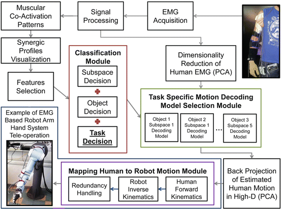
Fig. 1.13
A block diagram of the proposed EMG-based learning scheme is presented. Two main modules, formulate the “backbone” of the learning scheme, the classification module and the task specific model selection module. Classification module (based on the classifier) provides decision for subspace to move towards, object to be grasped and task to be executed with the object. Task specific model selection module (based on the regressor) examines classification decisions and triggers a subspace, object and task specific motion decoding model (from all possible models trained). The task specific motion decoding model efficiently estimates the full human arm hand system motion (27 joint values), using human myoelectric activity (EMG signals). Finally an EMG-based interface can take advantage of the proposed scheme and the estimated human motion. For example a human to robot motion mapping procedure may take as input the estimated human arm hand system motion, to generate equivalent robot motion, as described in [40]. A possible application of the proposed learning scheme, is the EMG-based teleoperation of a robot arm hand system
1.3.2 Multiclass Classification in the m-Dimensional Space of Myoelectric Activations (m-Number of EMG Channels)
As we have already noted, synergistic profiles depicted in terms of “boxplot zones” in Fig. 1.7 denote that there is a significant differentiation of muscular co-activation patterns for reach to grasp movements towards different positions and different objects placed at the same position. In order to be able to take advantage of this differentiation, we choose to discriminate the different reach to grasp movements in the m-dimensional space of the myoelectric activations (where m is the number of EMG channels), using the EMG signals to “decide” on the task to be performed (human intention decoding).
In Fig. 1.14 we present a typical classification problem of discriminating based on the myoelectric activity of 16 muscles of the human arm hand system, two different strategies for reaching and grasping a specific object placed in two different positions. Reaching, grasping and return phases are depicted. The top subplot presents the distance between the two classes in the 16-dimensional space (16 EMG channels are used). Such a distance, give us a measure of classes separability (i.e., how easily these classes can be discriminated). The bottom subplot, presents the evolution of classification decision over time. The accumulation of misclassified samples is reasonable for those time periods, when the distance between the two classes is small (i.e. begin and end of experiments, when human end-effector (wrist), is close to its starting position).
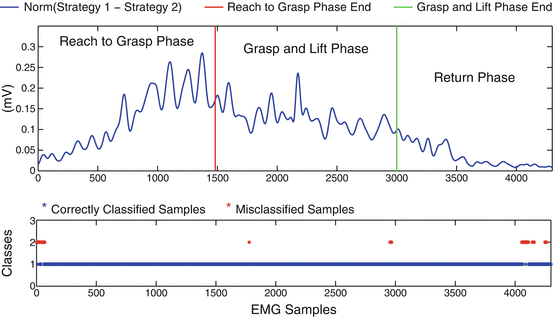
Fig. 1.14
Comparison of two reach to grasp movements towards a marker placed at position I (Strategy I) and a marker placed at position II (Strategy II). First subplot presents the distance of the two strategies in the m-dimensional space (where m = 16 the number of the EMG channels). The second subplot focuses on the evolution of classification decision per sample, over time
In Fig. 1.15 we present the classification problem of discriminating two different reach to grasp movements, towards a specific object placed at a specific position, but in order to execute two different tasks (with the object). Once again, top subplot presents the distance between the two classes in the 15-dimensional space (15 EMG channels are used), as well as the reaching, grasping and return phases. Bottom subplot presents once again the evolution of the classification decision and there is a similar with Fig. 1.14, accumulation of misclassified samples for the time periods, that the distance between the two tasks is small (i.e. begin and end of the experiment).
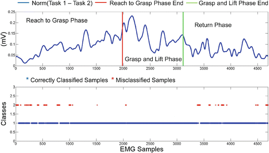
Fig. 1.15
Comparison of two reach to grasp movements, towards Position I to grasp a tall glass with two different grasps (side grasp and front grasp), to execute two different tasks. First subplot presents the distance of the two tasks in the m-dimensional space (where m = 15 the number of the EMG channels). The second subplot focuses on the evolution of classification decision per sample, over time
1.3.2.1 Random Forests Classifier
The Random Forests technique proposed by Tin Kam Ho of Bell Labs [44] and Leo Breiman [45], can be used for classification creating an ensemble classifier that consists of many decision trees. The Random Forests classifier’s output, is the class that is the mode of the individual trees class’s output. Thus, the classifier consists of a collection of tree structured classifiers {h(x, Θ N ), N = 1, …} where {Θ N } are independent identically distributed random vectors. Each decision tree of the random forest, casts a vote for the most popular class at input x.
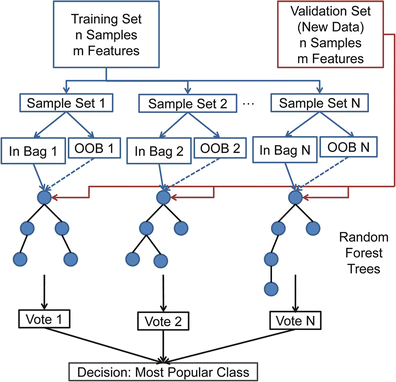
Fig. 1.16
Random forests based classification procedure for N trees grown. OOB stands for out-of-bag samples
The classification procedure for N trees grown is presented in Fig. 1.16. Some advantages of the random forests technique for classification are:
Runs efficiently and fast on large databases.
Provides high accuracy.
Does not overfit.
Provides feature variables importance.
Can handle thousands of input variables without variable deletion.
Can handle multiclass classification problems.
Can be used efficiently in multidimensional spaces.
1.4 Features Selection with Random Forests
In the aforementioned classification examples we used the random forests technique to discriminate, between different reach to grasp movements in the m-dimensional space of the myoelectric activations, using multiple EMG channels (m is 15 or 16). Its quite typical for EMG based interfaces, a limited number of EMG channels to be available (e.g., due to cost or complexity limitations), or EMG electrodes positioning to be not precise (some EMG channels may be more noisy). Thus, a fundamental question is: “Is it possible to select which EMG channels are the most important? How this features selection can be accomplished?”. With Random Forests we can perform efficient features selection, using their ability to compute the importance score of each feature variable and consequently access the relative importance for all feature variables (e.g., EMG channels).
More precisely random forests use for the construction of each tree, a different bootstrap sample set from the original data. One-third of the samples are left out of the bootstrap sample set (out-of-bag samples) and are not used in the construction of the Nth tree. Feature variables importance, is computed as follows; in every grown tree in the forest, we put down the out-of-bag samples and count the number of votes cast for the correct class. Then the values of a variable m are randomly permuted in the out-of-bag samples and these samples are put down the tree. Subtracting the number of votes casted for the correct class in the m-variable permuted out-of-bag data from the previously computed number of votes for the correct class in the untouched out-of-bag data, we get the importance score of a feature variable m for each tree. The raw importance score for each feature variable m is the average importance score for all trees of the random forest. The random forests feature variable importance calculation procedure, is depicted in Fig. 1.17.
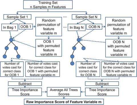
Fig. 1.17
Diagram of the random forests feature variable importance calculation procedure. OOB stands for out-of-bag samples
In case that we want to reduce the number of EMG channels used (in this study we have already used 15 and 16 EMG channels), random forests can be initially run with all the variables (EMG channels) and then run once again with the most important variables selected during the first run. For example, we can use the random forests classifier with all 15 EMG channels, compute the feature variables importance and re-solve the classification problem, using the most “important” EMG channels. Before doing so, we present the feature variables importance for the problems of discriminating from EMG signals, reach to grasp movements towards, different subspaces, different objects and different tasks.
In Fig. 1.18 we present the importance plots of different feature variables (EMG channels), for two different cases, subspace discrimination and object discrimination. We can notice that for subspace discrimination, the feature variables corresponding to upper-arm muscles (first 8 EMG channels) appear to have increased importance, while for object discrimination the feature variables corresponding to the forearm muscles (last 8 EMG channels), accumulate most of the importance.
Stay updated, free articles. Join our Telegram channel

Full access? Get Clinical Tree


