Fig. 16.1
The study-specific general linear model as created in SPM
Intermezzo: The Study’s General Linear Model
The water-activation-PET data was analysed in an imaging-specific data-analysis program called Statistical Parametric Mapping (SPM: www.fil.ion.ucl.ac.uk/spm/). In SPM the variance in the data is modelled using the General Linear Model (GLM). The GLM (Friston 1997) estimates parameters ‘β’ to explain the measured regional cerebral blood flow (rCBF) ‘x’ in terms of a linear combination of ‘K’ explanatory variables ‘g’ plus an error term:


Where
i = 1, …, I indexes the observations, i.e. all the scan of all the subjects.
j = 1, …, J indexes the voxel j of the images.
k = 1, …, K indexes the number of explanatory variables.
This can also be written in matrix form as X = Gβ + e
with
X the observation matrix
G the design matrix
β the parameter matrix
With every additional explanatory variable, the GLM will fit the variance in the data better as it has more degrees of freedom to do so. But using additional degrees of freedom will weaken the statistical power and therefore the possibility to find a significant result.
PET data has a limited number of observations and is therefore directly modelled via the ‘Basic models’ option. The data in the current study was modelled in SPM5 using a three-by-two-by-two factorial design representing three groups, two identity states, and two memory scripts. To this end, we first defined the default factor ‘Subject’ with the assumption of independent measures and, considering that multiple measurements were obtained for each subject, the error variance was assumed to be equal for this factor. Then the ‘Group’ factor (DID, CH, and CL) was set with the assumption of independent measures and with unequal variance since the groups were independent. The Identity and Script factors were combined in the ‘Condition’ factor representing the (simulated) identity NIS and TIS and the scripts t and n. Considering that multiple measurements were obtained for each condition within one subject, the error variance was assumed to be equal for this factor but the measurements are not independent. The GLM consisted of the three factor main effects: subject, group and conditions, and a group by condition interaction.
Objective measures were obtained at the end of each two-minute PET scan (blood pressure (systolic and diastolic) and heart rate (discrete and variability)). In addition, six subjective emotional measures were obtained (fear, sorrow, sadness, anger, shame, and disgust) and ten sensorimotor experiences (visual, kinaesthetic, auditory, olfactory + gustatory reactions, pain, physical numbness, body stiffening, paralysis, and restlessness). Including all these measures in the GLM to explain variance induced by autonomic reactions and suggestibility/simulation would absorb too many degrees of freedom. Therefore these measures were submitted to a Principal Component (PC) analysis, which ‘categorises’ variance into different components, i.e. eigenvectors. We used a cut-off of one for the eigenvalues. The variance in the subjective ratings could be described with the first two, six and five PC for the DID, high- and low-fantasy-prone groups, respectively, explaining 64, 68 and 72 % of the variance. The variance in the autonomic reactions could be described with the first three PC for each of the DID, high- and low-fantasy-prone groups, explaining 85, 82 and 87 % of the variance, respectively. These subjective and autonomic PC reactions were included as group-specific covariates of interest (mean padded). Finally, the global cerebral blood flow (CBF) was included as a nuisance covariate (AnCova by subject).
The full design matrix is presented in Fig. 16.1. From left to right the parameters included in the GLM can be read. The first factor ‘Subject’ allocates 27 columns and consists of the ten patients, the nine CH, and the eight CL and accounts for the subject specific variance. The next three columns define the second factor ‘Group’ consisting of the three groups and explain variance common to all groups. The factor ‘Condition’ consists of four columns and explains variance common to all four conditions: NISn, NISt, TISn, and TISt. The next 12 columns are the effects of interest as they account for the variance in the data that belongs to the Interaction of group × condition. The subtraction analyses described in this chapter are performed by setting the contrasts on these 12 columns. The next columns are the two sets of group-dependent physiologic and subjective measures covariates as created by the principal component analyses: DID two and three, CH three and six, and CL five and three. The last 27 columns accommodate variance due to differences in global cerebral blood flow (CBF), which was included as a nuisance covariate (AnCova by subject). Of note, alternatively a reduced design matrix can be used including only subjects, group × condition interaction, covariates, and the subject × gCBF (see also the tutorial at https://www.jiscmail.ac.uk/cgi-bin/webadmin?A2=spm;bbc7faf8.0805). This, however, does not change the results.
Reference
Friston KJ (1997) Analyzing brain images: principles and overview. In: Frackowiak RSJ, Friston KJ, Frith C, Dolan R, Mazziotta JC (eds) Human brain function. Academic Press, London, pp 25–41
16.2.3 Statistical Inference and Reporting
Our a priori hypothesis was that earlier findings would still hold after the correction for non-trauma-related factors. Both whole-brain and a priori region of interest (ROI) multiple comparisons correction were performed on the basis of false discovery rate statistics (Genovese et al. 2002). If an a priori hypothesised brain area did not survive whole-brain multiple comparison correction, i.e. only survived an uncorrected threshold of p < 0.001, multiple comparison correction was performed within the a priori region of interest (ROI) (Reinders et al. 2012). Note: In line with previously used statistical thresholds (Reinders et al. 2006), voxels surviving significant levels only uncorrected for multiple testing for the whole brain, i.e. p < 0.001, were reported as well, but for comparison purposes only. Only clusters larger than eight voxels are reported taking into account the spatial resolution of the PET camera. In contrast to the earlier publication (Reinders et al. 2012), here, only the most significant peak voxels in a brain region is reported for simplicity. Brain regions and Brodmann areas (BA) were defined using both the Talairach atlas (Talairach and Tournoux 1988) and Deamon (Lancaster et al. 2000). Activations in sulci were defined using Brain Tutor (www.brainvoyager.com).
16.3 Results
16.3.1 Comparing Simulated and Pathological Identity States
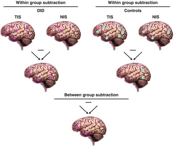
The comparison of different conditions in different groups is not always straightforward to understand. It can also be described as a between-group comparison of within-group differences. For clarification this is depicted in Fig. 16.2. The easiest approach is to think of this by starting with the within-group comparisons which can be performed for each group separately, as shown at the top of Fig. 16.2. Figure 16.2 shows a simplified graphical representation of the statistical comparison process and uses the conditions ‘NIS’ and ‘TIS’ as example conditions. These conditions can be replaced by, for example, TISt and NISt to clarify the between-identity state comparisons or by TISt and TISn to understand the within-identity state comparisons. The top row of Fig. 16.2 shows the two conditions in two groups. The middle row shows the result of the simple subtraction analyses between the two conditions within each group. The middle row therefore represents the within-group brain activation maps of the difference between the two conditions. These two differential maps are now compared to each other to obtain the between-group differential brain activation map, which is depicted on the bottom row. It is important to realise that the statistical model must start with a within-group comparison. Thus it is not possible to obtain meaningful results when directly comparing a single condition between groups. For example, we cannot investigate the difference for the NISt condition between the DID and control subjects.


Fig. 16.2
A between-group comparison of within-group differences. This figure depicts two conditions in two groups (DID and Controls) at the top row. The middle row shows the within-group differences of two conditions per group (DID or Controls). The bottom row depicts the between-group differential brain activation patterns. Note that SPM does not calculate each step separately; the figure is for clarification only
16.3.1.1 Within-Identity State Trauma-Related Memory Script Effects
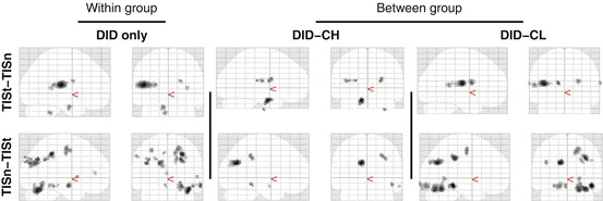
Trauma-related MS effects within both TIS and NIS are given in Table 16.1. TIS showed significant regionally specific increases and decreases in cerebral blood flow, when processing the trauma-related MS as compared to the neutral MS, between the DID and both the high- and low-fantasy-prone control groups. These findings are depicted in Fig. 16.3.

Table 16.1
Memory script effects within dissociative identity state
L/R | Brain regiona = a priori | Within group | Between group | ||
|---|---|---|---|---|---|
DID only | DID-CH | DID-CL | |||
TISt–TISn | |||||
Cortical areas | L | Insulaa | + | +c | +c |
L | Parietal operculuma | + | − | +c | |
R | Postcentral gyrus | − | − | + | |
R | I. temporal gyrus | − | + | − | |
L | S. temporal gyrus | − | − | + | |
Subcortical areas | L | Amygdalaa | + | +c | − |
L | Caudate nucleus (dorsal part)a | − | − | +c | |
R | Caudate nucleus (dorsal part)a | + | +c | +c | |
L | Caudate nucleus (tail)a | + | +c | − | |
R | Caudate nucleus (tail) | + | − | − | |
L | Putamen | − | + | + | |
Cerebellum | L | Cerebellar tonsil (nodule)a | + | − | − |
TISn–TISt | |||||
Cortical areas | R | Angular gyrus | − | − | + |
L | Anterior cingulate gyrus | + | − | − | |
L | Posterior cingulate gyrusa | + | − | − | |
R | Cingulate sulcusa,c | + | − | +b | |
L | Cuneusa | + | +b | − | |
R | Cuneus | + | − | − | |
R | I. frontal gyrus | + | − | − | |
R | Fusiform gyrusa | + | − | + | |
L | Lingual gyrus | − | − | + | |
R | Lingual gyrus | − | − | + | |
L | S. occipital gyrus/angular gyrusa | + | − | + | |
R | S. occipital gyrusa | + | − | − | |
R | S. occipital sulcus/cuneusa | + | − | − | |
R | Occipitotemporal sulcusa | + | + | +b | |
L | Parahippocampal gyrus | − | − | + | |
L | Intraparietal sulcusa | + | − | − | |
R | Intraparietal sulcusa | + | +b | +b | |
L | Rostral I. parietal lobulea,d | + | − | − | |
R | S. parietal lobule/precuneusa | + | − | +b | |
L | Precentral sulcusa | + | − | − | |
L | Precuneus | + | + | + | |
R | (Pre-)cuneus/parieto-occipital sulcus | + | − | − | |
R | M. temporal gyrusa | + | + | − | |
Cerebellum | L | Cerebellum (anterior lobe) | + | − | + |

Fig. 16.3
‘Glass brain’ renderings showing differences in the processing of the trauma-related text (indicated with a small ‘t’) and the neutral text (indicated with a small ‘n’) within the trauma-related identity state (TIS). Differences in regional cerebral blood flow patterns for the dissociative identity disorder (DID) group (left) and the comparison of this group to the high- (middle) and low (right)-fantasy-prone DID simulating controls (CH and CL, respectively) are depicted. See Table 16.1 for the specific areas
16.3.1.2 Between-Identity State Trauma-Related Memory Script Effects
Trauma-related MS effects between NIS and TIS are given in Table 16.2. Different rCBF patterns were found for NIS and TIS, when processing the trauma-related MS, between the DID and both the high- and low-fantasy-prone control groups. These differential rCBF patterns are shown in Fig. 16.4.
Table 16.2
Memory script effects between dissociative identity states
L/R | Brain regiona = a priori | Within group | Between group | ||
|---|---|---|---|---|---|
DID only | DID-CH | DID-CL | |||
TISt–NISt | |||||
Cortical areas | L | Insula | + | − | +b |
R | Insula | − | − | + | |
L | Orbitofrontal cortex | − | + | − | |
R | Parietal operculum | − | − | + | |
R | Postcentral gyrusa | + | + | +b | |
R | Precentral gyrus | − | − | + | |
L | S. temporal gyrus | − | − | + | |
Subcortical areas | L | Amygdalaa | + | +c | − |
R | Caudate nucleus (caudal part)a | + | +c | − | |
L | Caudate nucleus (dorsal part)a | + | +c | +b | |
R | Caudate nucleus (dorsal part)a | + | +c | +b | |
L | Caudate nucleus (tail)a | + | − | − | |
L | Putamena | − | +c | − | |
R | Putamen | − | − | + | |
Cerebellum | L | Cerebellar tonsil (nodule)a | +
Stay updated, free articles. Join our Telegram channel
Full access? Get Clinical Tree
 Get Clinical Tree app for offline access

| ||


