Epidemiology
Eric Fombonne
This chapter introduces the reader to basic concepts and terminology used in epidemiological research. In the first part, we illustrate how epidemiologists measure disease occurrence, design studies, and select samples to identify risk factors, and evaluate data to establish the causal nature of statistical relationships. In the second part, some achievements of 40 years of epidemiological research in child psychiatry are reviewed briefly. We first review issues specific to psychiatric epidemiology as they apply to the definition and assessment of child psychopathology in relation to the differentiation between normal and abnormal development, the use of dimensional or categorical approaches to case definition, the need to use impairment measures and to combine data from multiple informants, the need to take into account high rates of comorbidity between disorders, and the implications of pervasiveness or situational specificity of behaviors in estimating rates and risk associations for psychiatric disorders. Basic principles of measurement (reliability and validity) are defined as well as techniques used to screen and evaluate the performance of instruments. We then summarize findings on global psychiatric morbidity in children and adolescents as estimated from recent major population surveys and discuss issues relevant to special groups or new methodologies.
General Epidemiology
Definition and Historical Background
Epidemiology is the study of the distribution of diseases in human populations and of the factors that influence that distribution. The focus of epidemiology is to study patterns of disease occurrence in order to identify factors that are causally associated with the onset of disease in some individuals. Epidemiology relies essentially on observational (nonexperimental) methods. Descriptive epidemiology is mostly concerned with estimating rates of the disease for public health, or for administrative or monitoring purposes. Analytical or causative epidemiology concentrates on the identification of causes of disease occurrence in humans. Clinical epidemiology encompasses activities that use epidemiological methods to study other aspects of a disease, such as its natural history, factors that facilitate offset or persistence of the disorder, or relapse or other outcomes (i.e., mortality). One part of clinical epidemiology employs experimental methods (randomized clinical trials), where investigators can manipulate (through randomization) variables (treatments to which patients will be exposed) in designs that facilitate the derivation of causal inferences. Other types of epidemiology (genetic, occupational, psychiatric, …) are defined both by the substantive area of research and by appropriate modifications of epidemiological techniques and tools, although epidemiological concepts and theories remain essentially the same across domains of application. The rest of the chapter is concerned with observational studies.
Epidemiology started in the nineteenth century with studies of infectious diseases, such as with the discovery of the infectious nature and mode of transmission of cholera in a London epidemic. In psychiatry, early efforts at the turn of the twentieth century helped to uncover the carential nature of the pellagra encephalopathy; or ecological studies of suicide led to hypotheses linking suicide rates and social change. After World War II, major epidemiological studies contributed to the understanding of the risk for cardiovascular disease or demonstrated the causal association between smoking and lung cancer. Explaining this relatively recent development, epidemiological studies require the collection of large amount of data that may be difficult and costly to acquire. In the last 30 years, epidemiology has developed as an independent discipline, with its own set of concepts and approaches. Medical and biological knowledge and statistical techniques are used by epidemiologists but epidemiology goes much beyond the statistical analysis of medical data.
Measures of Disease Occurrence
Several measures of disease occurrence are used by epidemiologists. We define here the three most commonly used: incidence rate, cumulative incidence or incidence proportion, and prevalence.
Incidence Rate and Cumulative Incidence
To calculate incidence, individuals initially free of the disease must be observed over a period of time. The example in Figure 2.2.1.1 illustrate new onsets of disease (or death, or relapse, or any other health event) among six individuals observed during a period of ten units of time (i.e., months or years). Some individuals (subject 1) are observed for the whole observation period, whereas others (individuals 4 to 6) have reduced observation times as they join or leave the sample during the observation period. Three disease onsets (individuals 2, 3, and 5) are observed; for these individuals, the period of observation ceases when the event has occurred, as subsequently they are no longer at risk of developing the disease and the observation time following the event becomes uninformative. The length of the line for each individual in Figure 2.2.1.1 represents the person-time experience of this individual and its own contribution to the denominator of the incidence rate. Only events occurring in individuals who are contributing to the person-time denominator are counted.
The incidence rate (IR) is calculated as follows:
In the Figure 2.2.1.1 example, the incidence is IR = 3/36 = 0.083 time units-1. IR can vary from 0 to infinite. It has the inverse of time as a unit (i.e., 0.083 per year) which, under some circumstances, can be interpreted as an average waiting
time before disease onset. With a fixed number of events, the incidence increases if the person-time denominator decreases, as when the onset of new cases of disease occurs more rapidly, reflecting a faster penetration of the disease in the population. Calculation of incidence rates are more complex in real circumstances, depending on particular assumptions that hold true for the observed population (open [in steady state] or closed population, migration in or out, consideration of competing risks). Common examples of incidence rates are mortality rates, which have an easy intuitive meaning. For example, a young male suicide rate of 20/100,000/ year or 0.0002 year-1 means that, if one were to follow up 100,000 young males for a duration of one year each, 20 suicidal events would have been occurring during that observation period. However, the same incidence rate could be obtained with four suicidal deaths observed in following 2,000 subjects over a ten-year period. The numerical value of an incidence rate can therefore have different meanings depending on the study methodology.
time before disease onset. With a fixed number of events, the incidence increases if the person-time denominator decreases, as when the onset of new cases of disease occurs more rapidly, reflecting a faster penetration of the disease in the population. Calculation of incidence rates are more complex in real circumstances, depending on particular assumptions that hold true for the observed population (open [in steady state] or closed population, migration in or out, consideration of competing risks). Common examples of incidence rates are mortality rates, which have an easy intuitive meaning. For example, a young male suicide rate of 20/100,000/ year or 0.0002 year-1 means that, if one were to follow up 100,000 young males for a duration of one year each, 20 suicidal events would have been occurring during that observation period. However, the same incidence rate could be obtained with four suicidal deaths observed in following 2,000 subjects over a ten-year period. The numerical value of an incidence rate can therefore have different meanings depending on the study methodology.
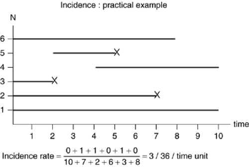 FIGURE 2.2.1.1. Calculating incidence. |
Because incidence rates are not always that easy to interpret, epidemiologists use other measures of disease occurrence such as cumulative incidence (or incidence proportion). This measure is generally used for a closed population observed over a fixed period of time, all subjects being free of the disease at the beginning of the observation period. For example, if nine of 100 siblings of autistic probands develop autism from birth (the beginning of the observation period) to age three, the cumulative incidence of autism in this high-risk sample would be reported as 0.09 or 9% over the first three years of life. Unlike incidence rate, this figure is a proportion, dimensionless, and varying from 0 to 1. To be interpreted correctly, this cumulative incidence must be reported in conjunction to the length of the observation period, as the cumulative incidence will vary as a function of the followup time. In the previous example, if the sample is followed further from age three to five, another six cases might be newly diagnosed with autism, leading to a cumulative incidence of 0.15 over five years of observation. The intuitive interpretation of cumulative incidence is that it represents the average risk of developing the disease in the population under study (i.e., the summation of individual risks across individuals from the study population). One variant of incidence proportion is survival proportion, which is the complement of incidence proportion (survival versus death, no recurrence versus recurrence) and is often used in clinical epidemiological studies.
Prevalence
Prevalence focuses on disease status of individuals within a population rather than on the pattern of onset of new cases in that population. Prevalence is not a dynamic measure and, contrary to incidence rate or proportion, no passage of time is required for its calculation. Prevalence is calculated as the proportion of individuals in a population who, at a given point in time, have the disease. Prevalence (P) is a proportion1 that is dimensionless and varies from 0 to 1. It is calculated as:
Prevalence incorporates in its numerator recent and past onsets of the disease, and therefore the duration of the disease will influence the prevalence. If the disease is rapidly lethal or if it can be cured rapidly, the number of diseased individuals at any time point will drop and so will the prevalence. Thus, a prevalence rate reflects not only the incidence of the disease but factors that are associated with other aspects of the disease process (availability of treatments, natural history, lethality, …). The relationship of prevalence to incidence can be estimated, under some circumstances, as:
Nc ≈ P ≈ I × D where D is the average duration of the disease, I the incidence,
N – Nc
Nc the number of cases in the population, N the population size and P the prevalence proportion. If the prevalence is small enough (i.e. <0.10), the formula simplifies to: P = I × D. As I and D have respectively time-1 and time as units, P is dimensionless; it is a proportion that varies from 0 to 1. Prevalence rates can be useful as descriptors of the morbidity due to specific causes. They are useful for planning health and educational services. In some circumstances, they may also help generate hypotheses about causal factors associated with disease onset.
In psychiatry, prevalence rates are often referred to specific time periods. For example, a subject who has experienced a major depressive episode during the last 12 months but has now remitted might still contribute to the numerator of a prevalence rate if prevalence in that study is defined as 12-months period prevalence. In this example, any individual who met criteria for depression at any time point during the 12 months preceding the survey date would be defined as a case that would contribute to the prevalence pool (the numerator). The most commonly used period prevalence rates are 3-, 6-, and 12-months prevalence rates. Prevalence rates for longer periods of time can be useful to capture events that are either rare or episodic. Because the onset of symptoms of psychiatric disorder are often difficult to determine, psychiatric epidemiologists have often used the concept of lifetime prevalence. Thus, any individual who would have experienced a major depressive episode at any point during his lifespan would be counted at the numerator of a lifetime prevalence rate estimate, irrespective of his current disease status, of the age of first onset and of the total number of depressive episodes experienced by this individual over his life span.
Study Designs
The goal of epidemiologic studies is to examine whether or not particular variables are associated with a variation in disease occurrence. These variables are commonly referred to as exposures, as in the example of prenatal exposure to alcohol increasing the risk of neurodevelopmental and behavioral
abnormalities in children. Exposures can be susceptibility genes, prenatal or later life exposure to biological factors, a positive family history, psychosocial stressors, cognitive style or capacity, specific life events, and so on. When exposure to a variable of interest is associated with a demonstrated variation in the risk of the disorder, this variable is referred to as a risk factor for that disorder. A risk factor is statistically predicting of the disorder, but this relationship may or not be causal. The design and analysis of epidemiological studies aims at identifying risk factors and at evaluating the causal nature of their association with the disorder of interest.
abnormalities in children. Exposures can be susceptibility genes, prenatal or later life exposure to biological factors, a positive family history, psychosocial stressors, cognitive style or capacity, specific life events, and so on. When exposure to a variable of interest is associated with a demonstrated variation in the risk of the disorder, this variable is referred to as a risk factor for that disorder. A risk factor is statistically predicting of the disorder, but this relationship may or not be causal. The design and analysis of epidemiological studies aims at identifying risk factors and at evaluating the causal nature of their association with the disorder of interest.
Cohort Study
In cohort (or incidence) studies, the starting point consists of selecting two cohorts of subjects initially all free of the disease (Figure 2.2.1.2A). One cohort has experienced the exposure (exposed cohort) whereas the other (reference) cohort has not experienced it (unexposed cohort). Then, the person-time experience is measured in each cohort and the incidence of the disease can be estimated in each. The incidence in the exposed and unexposed cohorts is then compared by calculating an incidence rate ratio (Figure 2.2.1.2B) that is not different from 1 if there is no association between the exposure and the incidence. Conversely, if the exposure is associated with an increased risk of the disease, the IRR will be higher than 1. When the measure of disease occurrence available is the cumulative incidence, the relative effect of exposure on the disease is estimated by the risk ratio, obtained by dividing the cumulative incidence in the exposed cohort by that from the unexposed cohort.
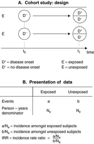 FIGURE 2.2.1.2. Design and presentation of data in cohort studies. |
Cohorts are defined by the exposure status of their members. Sometimes, one single cohort will be available, but measurement of the exposure for each subject will allow the construction of two or several cohorts according to exposure levels (unexposed vs. exposed; or nil, medium or high exposure). Cohort studies are difficult and costly to perform as they involve sometimes long periods of observation and therefore attrition can occur. One advantage of cohort studies is that several outcomes can be studied in relation to the initial exposure. Cohort studies are impractical if the disease incidence is low (rare disease), as the sample size required would be prohibitive. In some but not all studies, the investigator would be present at t0 and wait for the cohort to mature (t1) and live through the period at risk of developing the disease (prospective cohort study). In other studies (retrospective cohort study), the cohort study can be designed historically from data already collected. An example of this is the study showing a twofold increase in the risk of adult schizophrenia among subjects exposed to prenatal nutritional deficiency during the Dutch hunger winter in 1944–45 (1), a finding recently replicated for the Chinese famine in 1959–61 (2). Thus, the temporal position of the investigator regarding the data collection in a cohort study varies from study to study and is not what defines a cohort design. Knowledge of the biological mechanisms that might underlie an association and of the disease model under investigation are critical in designing cohort studies. Some exposures might have a long induction period (e.g., parental loss in childhood in relation to adult female risk of depression), which must inform the definition of the observational period and the data collection process.
Case-Control Study
In a case-control study, two groups are selected according to their present health status (with or without the disease of interest) and contrasted with respect to their past experiences of exposure to potential risk experiences (Fig. 2.2.1.3A). Case ascertainment must be as complete as possible in order to represent the full spectrum of the disease and to avoid selection biases, particularly when case sampling is not independent of the exposure. Cases can be selected from
the general population, but complete ascertainment may be difficult under these circumstances (i.e., identifying all cases of illness through hospitals, private clinics, and practices). Alternatively, cases may be selected in a cohort where more complete ascertainment can be achieved. Control selection is one of the most difficult design challenge in case-control studies. It is useful to conceptualize that the cases originated from a source population from which the controls should be selected, independently from knowledge of their exposure status. Controls should therefore represent adequately the distribution of the exposure in the source population from which cases originated. Only when this is achieved can the case-control analysis evaluate if the exposure experience differs meaningfully between the cases and the controls. An implication for this conceptualization is that it is usually wrong to select controls among healthy volunteers who are likely to underrepresent the frequency of exposure (supernormal controls or healthy worker effect in occupational studies) in the source population and bias upward the estimates of association. Approaches to the selection of controls that rely on friends, neighborhood, or classroom controls are appealing due to their convenience but may also pose threats to the validity. Numerous examples of such problems are found in the psychiatric or psychological literature, when patient data are compared to healthy volunteer data (i.e., referred depressed adolescents compared to high school students) or other convenient series of controls (classmates, friends, …) leading to spurious “positive” findings.
the general population, but complete ascertainment may be difficult under these circumstances (i.e., identifying all cases of illness through hospitals, private clinics, and practices). Alternatively, cases may be selected in a cohort where more complete ascertainment can be achieved. Control selection is one of the most difficult design challenge in case-control studies. It is useful to conceptualize that the cases originated from a source population from which the controls should be selected, independently from knowledge of their exposure status. Controls should therefore represent adequately the distribution of the exposure in the source population from which cases originated. Only when this is achieved can the case-control analysis evaluate if the exposure experience differs meaningfully between the cases and the controls. An implication for this conceptualization is that it is usually wrong to select controls among healthy volunteers who are likely to underrepresent the frequency of exposure (supernormal controls or healthy worker effect in occupational studies) in the source population and bias upward the estimates of association. Approaches to the selection of controls that rely on friends, neighborhood, or classroom controls are appealing due to their convenience but may also pose threats to the validity. Numerous examples of such problems are found in the psychiatric or psychological literature, when patient data are compared to healthy volunteer data (i.e., referred depressed adolescents compared to high school students) or other convenient series of controls (classmates, friends, …) leading to spurious “positive” findings.
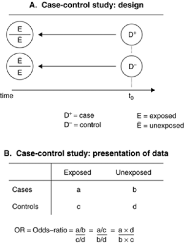 FIGURE 2.2.1.3. Design and presentation of data in case-control studies. |
To address the difficulty of control selection, two or more control groups may be selected that differ for their selection procedure and thus for the possible sampling biases that they each introduce. While intellectually appealing, this approach may be practically very labor intensive. Furthermore, there is no guarantee of the absence of bias when similar estimates are obtained when comparing the case series to each control group; conversely, if diverging estimates are obtained with each control group, the investigator is left with the difficult (and often impossible) task of determining where from and in which group the source of bias operates.
Exposure data are often (but not necessarily) collected retrospectively, making the study vulnerable to measurement biases due to differential recall (or recall bias) or missing data. For example, when interviewed and compared to nondepressed controls, currently depressed individuals might overreport past negative life experiences simply because their threshold for remembering and evaluating as negative particular events might be affected by their current mood state. Incidence rates are not available in a case-control study; estimates of the association between the candidate risk factor and the disease are calculated by comparing the odds of exposure among the cases and the controls (Figure 2.2.1.3B). One sometimes calculates the case/control ratio among exposed (a/c) and unexposed subjects (b/d), which leads mathematically to the same computation of the odds ratio. This calculation also illustrates how case-control studies converge toward cohort studies provided that the controls provide an adequate representation of the exposure distribution in the source population (i.e., when c and d converge towards Ne and Nē, (see Figures 2.2.1.2B and 2.2.1.3B). The resulting odds ratio (OR) is an estimate of the incidence rate ratio obtained in cohort studies. Case-control studies can be performed more rapidly and are efficient. They are particularly required for rare diseases. Case-control studies also allow for the evaluation of several exposures in relation to a given disease.
Cross-Sectional Study
Cross-sectional studies are studies of large and representative samples of populations at a given point in time. Usually, disease status and exposure status are measured at the same time, and these data can then be used to calculate prevalence rates and prevalence rate ratios. Prevalence rates can be informative for planning and services purposes. Prevalence rates can also be compared in various subgroups of the population (males vs. females, high or low SES, rural vs. urban, …) in order to identify characteristics or risk factors associated with disease status. Limitations of cross-sectional studies are that duration of the disease and other factors (earlier diagnosis, efficacious treatments …) unrelated to disease onset influence the size of the prevalence pool (see above).
Ecological Study
In ecologic (or aggregate) studies, the unit of observation is the group rather than the individual. The level of analysis could be classrooms, schools, neighborhoods, municipalities, states, or countries. If both exposure and health outcome data are available at that level of analysis, their relationships can then be examined. For example, county suicide rates could be positively correlated with county unemployment rates, suggesting that unemployment leads to suicide. However, the joint distribution of exposure and disease is generally not known at the individual level, and it is possible that those individuals who commit suicide are not those who are unemployed (e.g., suicide might be occurring among young people, whereas unemployment would affect those over age 50). This interpretation problem has been identified as the ecological fallacy or ecological bias. In these studies, information about confounding factors (age, in the previous example) is usually very limited; in addition, the temporal sequence between disease events and exposure (that must precede the health outcome) can be difficult to determine. Ecological studies have the advantage of being simple and cheap to perform considering the wide availability of vital statistics and sociodemographic indicators in many countries. Time trend analyses and crossnational comparisons are also forms of ecological studies that may yield useful information not readily available otherwise. Ecological analyses can also be informative in circumstances where levels of individual exposure lack variability (i.e., all individuals in a population are unexposed or all are exposed). For example, studies examining risk of autism in relation to exposure to vaccination might be uninformative if every child in the study population has been vaccinated. Comparing rates of autism in areas or time periods that differ for their rates of vaccine uptake (an ecological comparison) might be the most informative approach. For example, rates of pervasive developmental disorders (PDD) increased in Quebec from 1987 to 1998 but, as levels of exposure to thimerosal through vaccines varied from medium to high and then nil during the same period, investigators used this natural experiment to show that trends in PDD rates were unrelated to exposure to varying thimerosal levels (3). In some investigations, ecological effects are also the focus of interest even when individual-level data are available. For example, one might want to examine the respective contribution to the individual risk of engaging in antisocial behavior from both child and familial characteristics (individual level) and of community characteristics (group level). Multilevel analyses of that kind have often been conducted in the social sciences.
Other Designs
Other study designs or mixed designs can be used in epidemiology. For example, a case-control study can be nested in a cohort study, which provides opportunities to ascertain a representative sample of cases and of controls and to rely on prospective (less biased) measurements of risk factors. In that instance, the case-control study would be referred
to as a prospective case-control study owing to the fact that the measurement of risk factors precedes that of the onset of disease. Other study designs are discussed extensively elsewhere (4).
to as a prospective case-control study owing to the fact that the measurement of risk factors precedes that of the onset of disease. Other study designs are discussed extensively elsewhere (4).
Issues of Sampling and Data Analysis
Sampling
In large population-based cross-sectional surveys that have been typical of psychiatric epidemiology in the last 40 years, sampling techniques vary from simple random sampling (SRS) to more complex stratified or cluster sampling strategies that aim to increase the precision of estimates, while optimizing survey resources and reducing costs. A typical example of a complex survey design would be a survey where two strata defined by the type of classrooms (special education versus mainstream) are selected and children from special education classrooms are sampled with a higher sampling fraction than their counterparts. In addition, if all the subjects within each classroom are selected, the natural occurrence of these clusters must be taken into account, as observations are no longer independent (the same would apply to household surveys). For example, the same teachers would be providing data on several children who also happen to share common experiences that may be determinants of behavioral disorders (teaching quality, physical characteristics of the classroom).
In selecting children for inclusion in the study sample, it is crucial to note the probability of each child being selected, so that subsequently these probabilities can be used to weight back the observations (usually with weights that are the inverse of the sampling fraction) for extrapolation to the target population. This allows oversampling of some subgroups without distortion of the final estimates, provided that proper weights are devised and applied. Taking into account the clusters and strata used initially as sampling frames is also required in order to derive unbiased variance estimators. The analysis of two-phase or more complex survey designs is discussed further by Dunn et al. (5).
Registers or Population-Based Electronic Databases
Registers are data collection systems maintained by administrative or public health authorities over time to monitor health indicators. Several psychiatric case registers exist that have been used in epidemiological investigations. When well maintained, they can provide an easy way to access and an efficient sampling source, from which various case-control or cohort studies can be derived in no time. Thus, national health and psychiatric registers available in Denmark or the General Practitioner Database in the U.K. have been invaluable tools for epidemiologists to allow them to test rapidly emerging hypotheses, such as on the risk of autism in relation to exposure to measles-mumps-rubella vaccine, or to the thimerosal content of children’s immunizations. Different research designs were used from those sources, and including cohort (6,7), case-control (8) or ecological (9) studies, all of which failed to detect any association.
Sample Size and Precision
In each study, the goal is to estimate rates or measures of association with as much precision as possible. Precision is decreased by various sources of random error, including imperfect measurements of exposure or disease status (see below), or sampling errors. In order to limit the loss of precision due to sampling error, increasing the sample size is a common technique that involves detailed calculations at the designing stage of the study that consider cost of sampling, sample availability, and preliminary estimation (based on past studies or conceptual considerations) of the likely range of values for the rates differences or risk ratios to be estimated. A tradeoff between gaining more precision by increasing sample size and the expanding costs of the study is often a consideration. In some case-control studies, the study efficiency can be tremendously improved by selecting several controls for each case. This would apply to circumstances where the number of available cases is limited, more statistical power is required, and controls are ubiquitous and cheap to obtain. Matching up to four or five controls to each case would maximize the power of the study. Beyond that number, the gains of matching extra controls become rapidly smaller and not worth pursuing.
Missing Data
Methods for dealing with missing data are crucial and have been addressed more efficiently in recent surveys. Participation rates in child psychiatry surveys have generally been high, often well over 80%. Bias in the estimates of prevalence and risk associations might result, nevertheless, if those who do not participate have higher rates of disorders, more severe disorders or disorders arising through different mechanisms. Empirical findings indicate that nonrespondents often differ systematically from respondents. For example, in a survey of school-age children, behavioral disturbances reported by teachers were 60% higher among nonparticipants than participants, but survey weights could be used to correct for this bias in the final prevalence estimation (10). Similarly, attrition bias in longitudinal studies may attenuate predictions regarding the persistence of disorders over time (11).
Missing data can also occur at the item level, with respondents omitting items on a checklist or failing to answer all questions in an interview. This may jeopardize data collection (if incomplete screens are deemed ineligible for further interview) or analysis (if incomplete interviews are not dealt with separately). Sophisticated statistical and imputation techniques are available to take account of missing data, different according to the reasons that they are missing (12,13).
Statistical Testing
Point estimates of disease occurrence (incidence, prevalence) and of measures of association (relative risks, such as rate, risk and odds ratios) derive from the particular samples studied by investigators. The values obtained in one study are meant to be robust and unbiased estimators of the true population value, also called population parameters. In any one study, there is imprecision attached to each point estimate and epidemiologists communicate findings with 95% confidence intervals calculated around point estimates. For example, the odds ratio in a case control study could be expressed as: OR = 2.2 [95% confidence interval: 1.5— 3.4]. A 95% confidence interval can be construed around all measures of disease occurrence and of association reviewed earlier. Confidence intervals provide a range of values that are consistent with the true population parameter under the present study circumstances. For measures of association, a relative risk of 1 is the expected value under the null hypothesis of no association between the exposure and the disease. If a 95% confidence interval around a point estimate for the relative risk includes 1, the null hypothesis is not rejected. If 1 is not included in the 95% confidence interval (as in the above example), the null hypothesis is rejected at the 0.05 significance level. Too much emphasis is sometimes placed on statistical testing. Statistical testing is necessary in circumstances where decisions must be made (treat this patient or not). In most studies, epidemiologists are interested in evaluating causal relationships, and a probabilistic rather
than a black and white (significant or not) approach to this problem is warranted. Suffice it to remember that a very small effect (OR = 1.2; 95% CI: 1.05–1.45) of unlikely biological or clinical relevance could reach statistical significance only because the study has huge statistical power due to a very large sample size. Conversely, a larger, but statistically not significant, effect (OR = 2.9; 95% CI: 0.9–5.4) could point toward true associations of moderate magnitude. In those circumstances, epidemiologists who pursue causality will pay more attention to the strength of the association (the point estimate) and its interpretability in the larger context of the study design and findings. Causality assessment is better viewed as an ongoing, continuous, interpretative process that might be jeopardized with premature decision making rules embodied by classical statistical rules.
than a black and white (significant or not) approach to this problem is warranted. Suffice it to remember that a very small effect (OR = 1.2; 95% CI: 1.05–1.45) of unlikely biological or clinical relevance could reach statistical significance only because the study has huge statistical power due to a very large sample size. Conversely, a larger, but statistically not significant, effect (OR = 2.9; 95% CI: 0.9–5.4) could point toward true associations of moderate magnitude. In those circumstances, epidemiologists who pursue causality will pay more attention to the strength of the association (the point estimate) and its interpretability in the larger context of the study design and findings. Causality assessment is better viewed as an ongoing, continuous, interpretative process that might be jeopardized with premature decision making rules embodied by classical statistical rules.
Bias and Confounding
Whereas sample size can influence the precision of a study, sample selection can limit the validity of the estimates obtained by introducing systematic (as opposed to random) error in the rate or risk ratio estimates. Various other sources of bias are well recognized in epidemiology, which are also briefly described here.
Selection Bias
Selection bias occurs when subjects who participate in the study differ systematically from the population that they represent for characteristics associated to the disease or exposure under study. Several examples have been discussed above. One other example of selection bias is selective attrition when, in a cohort study, subjects who are lost to follow-up differ from the cohort subjects with respect to the incidence of the disease. Migration in or out of a population or differential mortality are similarly potential sources of bias. When selection biases of that kind are suspected, it is critical for investigators to use baseline data to empirically test whether or not subjects lost to followup are systematically different from those who are not. Selection biases are a particular concern in case-control studies, especially with respect to the selection of controls.
Information Bias and Misclassification
A valid measure of the association between the exposure and the disease depends on the accuracy of measurement of both variables. Due to measurement error, a diseased subject could be classified as control, or an unexposed subject as exposed. Measurement errors on dichotomous classifications of exposure and disease status are described with concepts of sensitivity and specificity (see below). Classification errors are referred to as misclassification and a more general discussion of measurement principles and errors as it applies particularly to psychiatric research is provided below.
In an epidemiological study where the goal is to estimate without bias an association, a critical feature of misclassification is whether or not it occurs independently of other variables. Differential misclassification occurs when the measurement error affects cases or controls, or exposed versus unexposed subjects, with different patterns. A typical example of differential misclassification is recall bias. For example, in a case-control study of a severe birth neurodevelopmental abnormality of unknown origin at the time, mothers of cases reported significantly more psychosocial stressors during pregnancy (financial difficulties, marital difficulties) than mothers of controls (14). This suggested that psychosocial stress could be a cause of the negative birth outcome. It turned out that the abnormality was Down syndrome, the chromosomal etiology of which was only discovered in the months that followed. The only explanation for the spurious association between Down syndrome and psychosocial stressors during pregnancy in Stott’s study lies in the differential reporting by mothers of cases (in search of a cause for their child’s anomaly) of their past psychosocial experiences. It is important to consider that measurement error itself is not the problem if it affects subjects across groups equally. The bias arises from the fact that cases and controls do not report their exposure experience in a comparable fashion. Recall bias is a well recognized problem of retrospective case-control studies that can be addressed and prevented. For example, obtaining evidence from other sources of information, preferably collected before the onset of the disease (past medical or educational records), or through informants who are blind to the case status of study subjects, would limit the possibility of differential misclassification. Differential misclassification can inflate measures of association as in the previous example, or they may also attenuate them.
Nondifferential misclassification occurs when classification errors on exposure or on disease occur independently of each other. This type of misclassification almost always attenuates measures of association and biases the study results toward the null hypothesis of no association between the exposure and the disease. For example, in a case-control study free of measurement error of 200 depressed adolescents compared to 200 nondepressed controls, the presence of two or more negative life events (LE +) compared to one or less events (LE -) in the 12 months preceding the onset of depression is a risk factor for adolescent depression, with the ratio of exposure (LE +/LE-) being 80/120 in the cases and 40/160 in the controls, which translates into an odds-ratio of 2.7 (see Figure 2.2.1.3 B). If one assumes now that life events are measured with an imperfect questionnaire method that misclassifies 20% of subjects truly LE + as LE – and 20% of truly LE – subjects as LE +, and that this occurs equally among cases and controls (the misclassification is nondifferential, as it is independent of disease status), the ratio of exposure (LE +/LE-) is now 88/112 in the cases and 64/136 in the controls, which translates into an odds ratio of 1.7. In this example, the odds ratio is biased towards the null value of no association due to an unwelcome mixture of exposed and unexposed subjects in both cases and controls that blurs the true contrast of exposure distribution that exists between cases and controls in the absence of measurement error. Similar biases would occur if nondifferential misclassification applied to disease status. In general, therefore, nondifferential errors must be discussed in relation to negative studies or studies with associations of small magnitude. Differences in the error rate of measurement across studies may explain inconsistent or discrepant findings. In psychiatry, reliance on questionnaires and interviews, on lifetime measures of risk or disease experience, and on broad diagnostic groupings, are potential sources of considerable misclassification.
Confounding
Confounding factors are variables that may be responsible for a distortion of the relationship between the exposure and the disease. As such, confounding factors might over- or underestimate an association, and sometimes may even change the direction of the association. Confounding variables operate in all aspects of research, including in experiments. However, methods exist in experimental research (e.g., randomization) to limit the distorting effects of confounding factors. In nonexperimental designs, the control of confounding factors may be more difficult to achieve. To be a confounding factor, a variable must be shown (or known) to be associated with both the exposure and the disease independently. Furthermore, a confounding factor cannot merely be an intermediate variable in the causal chain linking exposure to disease. In a study where smoking during pregnancy is associated with later behavioral problems in the child, maternal antisocial behavior is a likely confounding factor. Maternal antisocial behavior is associated to smoking during pregnancy, and quite separately, it is associated with increased risk of child behavioral problems independently of its association to maternal prenatal smoking. Thus, the association between prenatal maternal smoking and
later child behavioral problems could be entirely accounted by the confounding effects of maternal antisocial behavior. In other words, the cooccurrence of smoking and behavioral problems could be artefactual and entirely driven by their background association to maternal antisocial behavior.
later child behavioral problems could be entirely accounted by the confounding effects of maternal antisocial behavior. In other words, the cooccurrence of smoking and behavioral problems could be artefactual and entirely driven by their background association to maternal antisocial behavior.
Related posts:
 Child and Family Policy: A Role for Child Psychiatry and Allied Disciplines
Aggression in Children: An Integrative Approach
Psychodynamic Principles in Practice
Child and Family Policy: A Role for Child Psychiatry and Allied Disciplines
Aggression in Children: An Integrative Approach
Psychodynamic Principles in Practice
 Evidence-Based Practice as a Conceptual Framework
Suicidal Behavior in Children and Adolescents: Causes and Management
Integrating Behavioral Services into Pediatric Care Settings: Principles and Models
Evidence-Based Practice as a Conceptual Framework
Suicidal Behavior in Children and Adolescents: Causes and Management
Integrating Behavioral Services into Pediatric Care Settings: Principles and Models
Stay updated, free articles. Join our Telegram channel

Full access? Get Clinical Tree


