Estimating the Location of Brodmann Areas from Cortical Folding Patterns Using Histology and Ex Vivo MRI

Fig. 4.1

Plot of the mean of the absolute value sulcal depth or average convexity versus the standard deviation across the 435 subjects in the OASIS dataset (Marcus et al. 2007)

In order to investigate the relationship between folding patterns and architectonic location, we used the reconstructed histological volumes provided by Drs. Amunts and Zilles to generate surface models of the gray/white interface for each of the subjects that they had obtained histologically-defined architectonic labels (Dale et al. 1999; Fischl et al. 1999a; Fischl et al. 2001). The 8 labeled Brodmann area maps (areas 2, 4a, 4p, 6, 44, 45, 17 and 18) were sampled onto the surface models for each hemisphere, and errors in this sampling were manually corrected (e.g. when a label was erroneously assigned to both banks of a sulcus). The 10 left and 10 right hemispheres were morphed into register using the high-dimensional nonlinear morphing technique that aligns cortical folding patterns (Fischl et al. 1999b) as described above, with heteroscedastic variance estimates. Note that no specific optimization was performed for aligning the Brodmann areas presented in this report. Rather, a set of parameters that had been determined to be optimal for aligning V1 in a separate ex vivo data set (Hinds et al. 2008) were used with no modification.

Using the surface-based registration, we constructed spatial probability maps for the 8 Brodmann areas. The results of this analysis are shown in Fig. 4.2, which displays the average convexity of the in vivo atlas that is used as a common space in dark (sulci) and light (gyri) gray, with the probability maps overlaid using a heat scale. These include primary and secondary visual areas BA 17 and BA 18, respectively, BA 44 and BA 45 (subdivisions of Broca’s area), somatosensory area BA 2, primary motor areas 4a and area 4p, and finally the premotor area BA 6. Frequency estimates of the probability that each point was part of each BA were constructed in a surface-based coordinate system by tabulating the number of times that a label occurred at a given point and dividing by the total number of subjects for each label. Each point in the surface-based coordinate system can then be probed to determine the probability that it is part of any of the set of labeled BAs. As can be seen, the folding-based surface alignment also results in extremely accurate alignment of the underlying BAs, particularly primary visual, somatosensory and motor cortex, thus highlighting the utility of the surface-based coordinate system as the space in which to develop techniques designed for the automated detection of architectonic boundaries in the human cerebral cortex.

A perfect coordinate system with respect to the architectonics would yield probability maps that are step functions – perfect certainty that a given coordinate is contained within an area transitioning to perfect certainty that one is outside an area. Unfortunately, current volumetric coordinate systems in use in neuroimaging are far from this ideal, yielding spatial probability maps with few if any coordinates that achieve perfect agreement in the training data (e.g. (Geyer et al. 1997; Amunts et al. 1999; Amunts et al. 2000; Geyer et al. 2000; Rademacher et al. 2002)). In contrast, the maps shown in Fig. 4.2 contain significant regions of 100 % probability, validating and quantifying the use of folding patterns to estimate the location of architectonic boundaries, a procedure that has been in use for decades.

In order to quantify the distance error in the folding-pattern-based registration, we used the registration to map the Brodmann Area labels across subjects and computed the symmetric mean Hausdorff distance between the mapped label and the true one, as shown in Fig. 4.3. The Hausdorff distance is a set-theoretic metric that measures the minimum distance from each point in one set to any point in the other, then typically is assigned the maximum over all points. Symmetrizing it means returning the average in each direction (i.e. the min using set 1 as the source and set 2 as the target, then the min using set 2 as the source and set 1 as the target). The mean Hausdorff distance uses the mean over all minimum distances as opposed to the max, and gives a better intuitive estimate of how close the majority of one boundary is to the other. Examining Fig. 4.3 we can see that in general the folding patterns are excellent estimators of the areal boundaries for primary motor and somatosensory areas, with V1 exhibiting an average boundary error of approximately 2.3 mm, or less than the size of a typical functional MRI (fMRI) voxel, with the estimation error increasing as one transitions up the putative cortical hierarchy to over 6 mm for BA44 and 45 in the left hemispheres, and even more than that in the right.

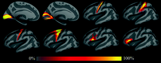
Fig. 4.2

Spatial probability maps of different Brodmann areas. Top row: left hemisphere areas 17, 18, 4p and 2 (from left to right). Second row: areas 4a, 6, 44 and 45. Third row: color scale used for spatial probability maps

4.2.2 Using Optimal Weighting of Cortical Folding Patterns

In the previous section we showed that the alignment of cortical folding patterns produced significantly better registration of the underlying architectonics than standard volumetric techniques. The underlying algorithm used to generate this result computes summary statistics from a population of subjects, then models the folding patterns using a Gaussian distribution, with the mean and variance of the Gaussians estimated from the training data at each point on the surface. The maximum a posteriori estimate of the registration function uses the inverse of the variance of the folds as a natural weighing. While the inverse variance is optimal for aligning folds given this specific probabilistic model (Gaussian distributed mean folding patterns), there is no reason to expect it to optimally align the underlying architectonics. In this section we discuss a recently developed computational technique to compute a weighting that is optimal for architectonic alignment.

Specifically, in the registration one uses the cross-subject mean image as a target, weighted by the cross-subject variance. In (Yeo et al. 2010) we generalized this method to learn both a target to replace the mean, and an optimal weighting to replace the inverse variance. The learning of such a set of patterns is extremely computationally intensive as for each step in the learning process all the training data must be registered with the current target and weighting, then the target and weighting are adjusted to more optimally align the architectonics, then the registration is run again and the process is iterated until it converges. However, while the training is slow, the use of the generalized target and vertex-wise weighting to register a new subject is exactly the same computational cost as the inverse variance weighting presented in the previous section.

The results of learning such a target and weighting and a comparison with the inverse variance weighting is given in Fig. 4.4. The red outlines in this figure represent the true outline of the underlying architectonic region as provided by histological analysis ((Amunts et al. 2000) for V1 and V2, (Amunts et al. 1999) for BA44 and 45, (Geyer et al. 1997; Geyer and Ledberg 1996) for area 2, and (Malikovic et al. 2007) for MT/V5), while the green outline shows the subject with the median accuracy for inverse variance weighting with a mean target (top row) and for optimal target/weighting in the bottom row. (Fig. 4.4)

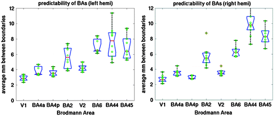
Fig. 4.3

Hausdorff distance from predicted boundary to true boundary for the left hemisphere (on left) and right hemisphere (on right) of ten subjects for eight histologically defined Brodmann Areas

Fig. 4.4

Localization provided by inverse variance weighting (top row) and optimal weighting (bottom row). Red outline is the true (histologically-based) Brodmann Area, and green is the one provided by the registration. The subject was chosen to be the one with the median accuracy of each technique. From left to right: V1, V2, MT/V5, BA2, BA44, BA45

Directly comparing the methods in terms of their mean symmetric Hausdorff distance in Fig. 4.5 reveals the increased accuracy of the computed optimal weighting with respect to the geometric weighting by inverse variance.

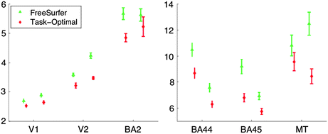
Fig. 4.5

Mean symmetric Hausdorff distance for inverse variance weighting (“FreeSurfer”, green) and optimal weighting (red). Note the different scales on the two plots, reflecting the accuracy of the alignment of areas closer to the sensory periphery (left) than those further in way in terms of number of synapses

4.3 Using Ex Vivo MRI to Visualize Architectonic Boundaries

In MRI one pays a steep price for increased resolution, a fact of imaging physics that has made the quest for high-resolution images a difficult one. The signal in a voxel is proportional to its volume, and therefore goes down with the third power of the length of the sides of an isotropic voxel. Isotropic voxel resolution is of course important so that we do not preference an arbitrary direction in the brain. In addition, signal-to-noise ratio (SNR) goes up with the square root of time, assuming temporally uncorrelated noise in subsequent acquisitions. This implies, for example, that to obtain the same SNR at ½ mm isotropic as at 1 mm isotropic, one must scan (2³)² = 64 times as long! It is therefore easy to see that simply scanning longer to recover the SNR required to get to high resolutions is not a tenable strategy. What resolution do we require to directly visualize histological properties suitable for detecting and labeling architectonic boundaries? If the cortex averages 2.5 mm in thickness, then each of the six layers is approximately 400 μms thick (although the total thickness is by no means equally distributed among the layers), and Shannon’s sampling theorem would suggest that 200 μm would be the coarsest resolution at which resolving the layers is possible. In practice, given the unequal laminar and spatial distributions of thickness we estimate that 100 μm resolution is required over much of the cortex. Given the basic physics relating SNR and resolution it is apparent that obtaining the resolution required to begin to visualize architectonic properties is exceedingly challenging.

It is worth pointing out the importance of developing techniques for delineation of areas with ex vivo MRI. The statistical modeling of relationships between macroscopic features and microscopic boundaries would benefit greatly from the availability of large numbers of examples. The handful that are available currently are simply insufficient, for example, to examine whether second order properties of the folding patterns are predictive of underlying cytoarchitectural boundaries. As one example: Do pairs of folds predict the location of an area, or, if tension based theories of morphogenesis (Van Essen 1997) have explanative power, then are the location of an area such as MT constrained by the locations of V1, to which it is directly connected, as well as the posterior callosum, through which fibers connecting MT to the contralateral MT flow? These and other questions can only be addressed if we have sufficient sample sizes of detailed structural/cytoarchitectural data, something that will be far easier to accomplish if we can directly image the necessary architectonic details without requiring mounting and staining of tissue sections.

While histology remains the gold standard of neuroanatomy, high resolution ex vivo imaging is gaining increasing importance (Johnson et al. 1986; Johnson et al. 2002; Augustinack et al. 2004; Hinds et al. 2008; Fischl et al. 2009; Yushkevich et al. 2009; Augustinack et al. 2010; Augustinack et al. 2012). While it is unlikely that ex vivo MRI can approach the types of resolution or specificity one obtains under a microscope in the near future (e.g. < = 1 μm), a series of factors make it feasible to increase SNR by up to three orders of magnitude relative to in vivo scans, an increase that can be directly traded for an order of magnitude in resolution. These factors include the lack of blurring induced by cardiac and respiratory cycles, the fact that small coils can be placed within a cm or so of the sample with no intervening skull to attenuate the signal and load the coil, and of course the possibility of scanning for many days as a means of recovering SNR is perfectly feasible (as opposed to the 90 min or so that is the maximum length of an in vivo scan session). Relative to histology, ex vivo MRI has some notable advantages:

It is possible to obtain multiple contrasts of the same exact tissue (e.g. T1, T2, proton density, diffusion, magnetization transfer, etc.….).

Obtaining whole-brain or whole-hemisphere MRI data requires no more effort than a small sample, and importantly, orders of magnitude less effort than whole brain histology.

MRI is an intrinsically three dimensional technique that yields isotropic voxels.

MRI does not incur irreversible distortions such as the tearing and warping induced by cutting, mounting and staining in histology.

These last two points are of particular importance, as they facilitate the accurate processing of large samples, including whole hemisphere and whole brains, something that is difficult or impossible to do with histological samples in with each section has been distorted differently, and the two in-plane directions are fundamentally different than the through-plane one. This is of particular importance when looking for discontinuities in the through-plane direction, or for example when trying to track axons or fascicles through-plane. An example of the types of data that one can acquire with ex vivo MRI together with the anatomical structures that are visible in it is given in Fig. 4.6.

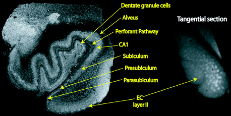
Fig. 4.6

Image of the human medial temporal lobe (left) acquired at 7 T with 100 μm isotropic voxels (TR = 20, TE = 5, α = variable). Right: oblique slice of same specimen through layer II of EC showing the layer II islands as brighter regions. Layers in the CA fields of the hippocampus and the dentate gyrus are clearly visible

In order to assess our ability to automatically detect architectonic boundaries with ex vivo MRI, we sampled the MRI data along line segments connecting the gray/white boundary and the pial surface throughout the extent of the sample. Independently, a neuroanatomist with great expertise in the medial temporal lobe (Dr. Jean Augustinack) manually delineated the borders of a set of medial temporal lobe regions including entorhinal cortex, parasubiculum, presubiculum and the subiculum proper (see Fig. 4.7). We then computed the distance between the laminar distribution of intensities along the line segments, ordering them from lateral to medial, and compared them with the manually defined borders, as is done in the histological processing shown previously (Schleicher et al. 1999). The results of this study are given in Fig. 4.8. As can be seen, each of the manually defined borders coincides with peaks in the distance function, indicating that these borders can be detected using the high resolution ex vivo MR data.

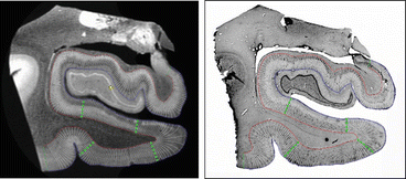
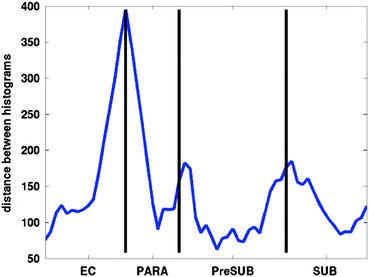
Fig. 4.7

Line profiles shown over a high-resolution 7 T ex vivo MRI (left) and the Nissl stain of the corresponding slice (right). The green lines show locations of local maxima in the properties of adjacent blocks of line profiles (red line = gray/white boundary, blue line = pial surface, Abbreviations: EC, entorhinal cortex; PC, perirhinal cortex; para-sub, parasubiculum; pre-sub, presubiculum)

Fig. 4.8

Distance between adjacent histograms of laminar intensity profiles from lateral (left) to medial (right). Note the peaks in profile distances indicating dissimilarity between the laminar distribution of intensities at manually defined border of EC and the para subiculum (PARA), the PARA and the pre subiculum (PreSUB), as well as the PreSUB and the subiculum (SUB) proper

Thus, these types of data can be used to build models of anatomical structures and infer the locations of architectonic boundaries in much the same way as the histological data has been. An example of this type of procedure applied to the boundaries of entorhinal cortex is given in Fig. 4.11. In the next section we discuss the challenges of acquiring MRI data ex vivo, and the types of image acquisitions that are optimal for fixed tissue.

4.3.1 Optimizing Image Acquisition and Reducing Distortions

The imaging of ex vivo tissue samples at high field involves different challenges than those posed by more standard in vivo structural imaging. The samples are almost always imaged after fixation, a process that dramatically changes their MR properties. Specifically, fixation reduces the T1 relation time of both gray and white matter, and brings them closer to each other. The result of this reduction is to make standard T1-weighting an extremely inefficient way to image fixed tissue samples. Here, we build on techniques we have developed for high SNR, low distortion imaging (Fischl et al. 2004) and adapt them for use in ex vivo samples with the goal of generating sufficient CNR to extend the number of cytoarchitectonic borders visible in MR images.

4.3.1.1 Optimizing Ex Vivo MRI Acquisition

Much effort has been devoted in the MRI community towards finding pulse parameters that are optimal for various tasks (Grief et al. 1985; Edelstein et al. 1986; Baker 1991; Constable and Henkelman 1991; Epstein et al. 1994; Constable et al. 1995; Venkatesan and Haacke 1997), including optimization for segmentation (Prince et al. 1995). In recent work, we phrased the segmentation problem in terms of models of image acquisition (Fischl et al. 2004). An advantage this type of approach is that it provides a natural framework for formulating an energy functional for sequence optimization specifically for segmentation. In particular, we can compute the probability of mistakenly labeling a voxel as class c ₁when the true class is c ₂as a function of the MR parameters m, using information from a probabilistic atlas:

$p({c_1}(\mathbf{r})|{c_2}(\mathbf{r}),\mathbf{m})=\int {p({c_i}(\mathbf{r})|\mathbf{I}(\mathbf{m}))p(\mathbf{I}(\mathbf{m})|{c_2}(\mathbf{r}))d\mathbf{I}=} p({c_1}(\mathbf{r}))\int {p(\mathbf{I}(\mathbf{m})|{c_i}(\mathbf{r}))p(\mathbf{I}(\mathbf{m})|{c_2}(\mathbf{r}))d\mathbf{I}}$

We then seek the combination of MR parameters m that minimize the probability of misclassification over all pairs of tissue classes that occur together anywhere in the atlas:

$\hat{\mathbf{m}} =\mathop{{\arg \min }}\limits_{\mathbf{m}}A(\mathbf{m})=\int\int\int\limits_{\mathbf{r}} {\sum\limits_{{{c_2}\ne {c_1}}} {\sum\limits_{{{c_1}}} {p(} } }{c_1}|{c_2},\mathbf{m},\mathbf{r})d\mathbf{r}$

The likelihood terms p( I |c _i( r )) are assumed to be normally distributed with means and covariances given by:

${{\hat{\mu}}_c}(\mathbf{m},\mathbf{r})=S({{\mathbf{m}}_{\mathrm{ predicted}}},\beta ({{\mathbf{m}}_{\mathrm{ training}}},{\mu_c}(\mathbf{r})),\;{{\hat{\Sigma}}_c}(\mathbf{m})={J_{\mathrm{ predicted}}}(J_{\mathrm{ training}}^{+}{\Sigma_c}J_{\mathrm{ training}}^{+T })J_{\mathrm{ predicted}}^{\mathrm{ T}}+\lambda Id$

where m _training are the MR parameters used in the construction of the atlas, and m _predicted are the MR parameters of the synthesized image being assessed, and the function S is the solution to the steady state Bloch equations (Bloch et al. 1946). The covariance structure is predicted by decomposing the noise into two parts. The first is anatomical variability in the intrinsic tissue properties of the various brain structures. The second is white noise inherent in the imaging process. In this formulation, J is the jacobian matrix of S, J ⁺ denotes the pseudo-inverse of matrix J, Id is the identity matrix, and λ is a constant that reflects the component of the noise that is scan-dependent, encapsulating factors such as averaging multiple acquisitions and the bandwidth of the scan. Numerically, equation (1) is integrated over the region of intensity that is nonzero for both classes c ₁and c₂, typically + −5 standard deviations from the mean. Minimizing equation (2) thus amounts to reducing the amount of overlap of the distributions for tissue classes that are likely to occur at the same location.

The ambiguity measure captures the difficulty of segmentation in several crucial ways. First, it allows the intrinsic properties of the tissue classes to vary over space, as the ambiguity is computed separately for each atlas location. This is important, as the tissue characteristics show considerable spatial variability (Ogg and Steen 1998; Steen et al. 2000; Fischl et al. 2004). Second, only tissue classes that co-occur in a given atlas voxel contribute to the ambiguity. Thus, the difficulty of segmenting for example cortical gray matter from dura would affect the sequence optimization, but not cortical gray matter from the caudate, as these structures never occur in the same region of atlas space. Finally, acquiring datasets for each of the possible parameters would not be tenable, something that is obviated by the use of the forward model of image formation S.

The parameter estimation procedure is based on a standard gradient echo saturation recovery acquisition protocol such as FLASH/SPGR, which is available on the vast majority of clinical scanners. As such, this sequence is limited in that it doesn’t take advantage of recent advances in imaging hardware and acquisition techniques. In particular, it is typically relatively low bandwidth, implying that distortions due to magnetic field inhomogeneities and susceptibility artifacts can be substantial. The low bandwidth is of course used to increase SNR. In general, there is a trade-off between high-bandwidth, low distortion, low SNR images, and low-bandwidth, high-distortion, high-SNR images. That is, SNR and distortion both go down with bandwidth.

In order to avoid this trade-off, we have developed a high-bandwidth multi-echo flash (MEF) sequence that minimizes distortion while maximizing SNR (Fischl et al. 2004). In a single 6.5 min scan, the same amount of time required for a 1 × 1 × 1 mm single-echo FLASH scan, this sequence provides 8 high-bandwidth images at different echo times. While the individual scans can be noisy, the information in the ensemble is significantly greater than the low bandwidth FLASH scans. In addition, the higher bandwidth of the MEF sequence, coupled with the fact that alternating echoes are collected with opposite read-out directions, results in less distortion in the images due to B0 effects (chemical shift and susceptibility distortion) (Fischl et al. 2004). This is particularly important for longitudinal studies in which different shim settings can result in substantial differential distortions between scan sessions for low bandwidth sequences. Physiologic and bulk motion during the readout also result in fewer artifacts due both to the shorter readouts of the multi-echo sequence, and to the averaging of the readouts with alternating directions. Finally, image reconstruction techniques can exploit the alternating readout direction to recover parts of the image previously lost due to susceptibility artifacts (Kadah and Hu 1998; Chen and Wyrwicz 1999; Schmithorst et al. 2001), an important consideration given the difficulty of removing all air bubbles when preparing an ex vivo sample of imaging.

We have recently developed a set of techniques for using MEF scans acquired at varying flip angles and/or repetition times (TR) to estimate the underlying tissue parameters that are the source of image contrast in standard gradient echo sequences (i.e. T1, proton density PD and T2*) (Fischl et al. 2004). Once these parameters have been estimated, they can then be used as input to simulations designed to maximize CNR noise per unit time. We applied these techniques to a set of ex vivo tissue samples, imaged in a 3 turn solenoid coil (28.5 mm i.d. × 44 mm in length) on a 7 T human scanner (Siemens Medical Systems, Erlangen, Germany). The data was acquired using a MEF sequence, with TR = 40 ms, α = 15°^,20°^,25°, 4 echoes, TE = 8 ms, 16 ms, 24 ms, 32 ms) at 100 μm isotropic resolution. The multiple flip angles were used to estimate the T1 and proton density of the underlying tissue using the techniques described in (Fischl et al. 2004). In addition, the multiple echoes were used to estimate T2^* using a log-linear fit to the data. ROIS were then manually drawn in the gray and white matter, and the mean tissue parameters were computed to be: T1 = (770 ms, 1078 ms), PD = (18,024,19,996), T2^* = (11 ms, 26 ms) for (wm,gm)). An example of the data (first 4 images) and the parameter maps (last 3 images) is given in Fig. 4.10. Interestingly, the dominant source of contrast in these images is given by T2* differences in the tissue.

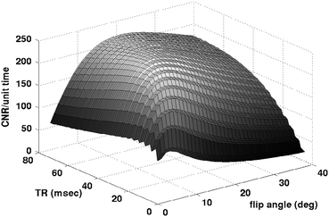
Fig. 4.9

Plot of CNR/unit time versus TR and α for ex vivo MEF

Fig. 4.10

Multi echo flash (images 1–4) with fitted T1 (image 5), PD (image 6) and T2^* (rightmost image)

Using these parameters, the steady state Bloch equations were applied (Bloch et al. 1946) and the CNR was computed over TR = [5,80], and flip angle α = [3,40]. For each TR/α pair, the CNR was computed by averaging the synthesized echoes, using an echo spacing of 3 ms, and assuming that 2 ms are required for spoiling at the end of each TR. The CNR was assumed to increase with the ½ power of the # of echoes that can be acquired for a given TR and echo spacing, and to decrease with sqrt(TR), corresponding to the assumption that the noise is time-independent (that is, a longer TR implies that fewer scans can be collected and averaged to increase SNR). Note that one advantage of the multi-echo FLASH is that bandwidth effects are no longer important, as the bandwidth is fixed at the maximum value in order to be continually reading data during the sequence. The optimum acquisition parameters from this simulation were computed to be TR = 48 ms, α = 16, which we will use in future acquisitions. One point to note is that this analysis does not take advantage of the change in contrast properties with echo time. That is, equal weighting of the echoes is clearly not optimal, as the contrast evolves in time due to the differing T2* properties of gray and white matter, as can be seen in Fig. 4.9.

Only gold members can continue reading. Log In or Register to continue