from the Past: Postprocessing of Classification Scores to Find a More Accurate and Earlier Movement Prediction

Fig. 1

Example data from single subject prior to a movement. Depicted are 4 s of data with the movement onset at the very right (0 ms). (a) The bold black line shows the median of all recorded epochs. Dashed lines are ten exemplary single trials. (b) Data of the same subject as (a) illustrated as 32/68 percentiles (black) and 5/95 percentiles (dark grey). The white line denotes time ranges where the data is labelled differently for evaluation: no movement (no mv) from − 4, 000 ms to − 1, 050 ms and movement (mv) from − 50 ms to 0 ms. In between, data is ignored for true labels (see text)

The question now is whether we can use the knowledge about this rise in classification scores to make the prediction more stable and/or predict the upcoming movement earlier. In trying to answer this question we were seeking for a postprocessing method that dampens fast fluctuations in classification scores and stabilizes long rises. To this aim, we applied several methods that modify the current classification scores by taking into account previous scores with a certain weight (see Sect. 2). To demonstrate the applicability and the benefit of these methods, we use all investigated methods in two simple ensemble approaches directly integrated in the signal processing chain (Sect. 6).

To summarize, if an LRP can be detected by high levels of the classification score, it could potentially just as well be predicted earlier by detecting the rise that leads to that elevated level. In the following we will describe the postprocessing methods that we have applied. After a description of the experimental data used, the results will be presented and discussed.

2 Postprocessing Methods

From the perspective of a movement prediction application it is most desirable to perform robust, binary decisions: A movement will either occur or it will not. This decision should be made as reliably and early as possible. From the large margin classification perspective, this means that the classification score S _tat some point in time t would have to be compared against some threshold b so that a movement mv is predicted when

$\displaystyle{ \mbox{ mv iff }\quad S_{t} \geq b. }$

(1)

Yet, as illustrated in Fig. 1, the score sometimes suddenly crosses the threshold when the actual movement is still far away, but then only for a short time. This behaviour hinders reliable prediction when it is purely based on the raw value of S _tcrossing b. Looking at the average score progression over time reveals a continuous rise of the score values before the actual movement. Here, we exploit this systematic behaviour to find a function F that is able to generate better movement predictions based on past values of S, such that

$\displaystyle{ \mbox{ mv iff }\quad F(S_{t},S_{t-1},\ldots,S_{t-(k-1)}) \geq b_{F} }$

(2)

for some specific threshold b _F. k is defined as the number of scores that are used in F with the current score being at k = 1. In principle, there are no constraints on the functional form of F.

In the present study we apply weights to the current and previous k − 1 classification outcomes to transform the current score S _t. These weights decay with the number of steps looked into the past. We also followed an alternative approach by transforming the current score with the average slope of the past samples. A detailed description is given in Sect. 2.2. Both types of functions (weighting and slope approach) can be expressed as

$\displaystyle{ F(S_{t},S_{t-1},\ldots,S_{t-(k-1)}) = w_{1}S_{t} + w_{2}S_{t-1} +\ldots +w_{k}S_{t-(k-1)} }$

(3)

with some predefined weights w. With this methodology we try to boost the score value when previous scores were similar in value and at the same time penalize scores when previous ones showed a completely different trend. The approaches are described in more detail in the following.

2.1 Fixed Weighting

In this set of functions the weights are generated by very simple functions, each of which assigns a high weight to the most current classification score sample, and decreasing weights to older samples.

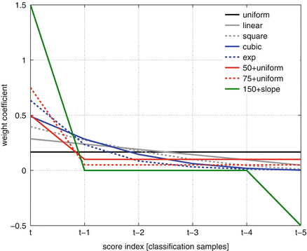
The functions used are depicted in Fig. 2. All functions have in common that the weights add up to one. The coefficients for the uniform, linear, square, and cubic method are all generated by evaluating

$\displaystyle{ w_{\tau } = \frac{\tau ^{p}} {\sum _{i=1}^{k}i^{p}},\quad \tau \in \{ 1,\ldots,k\}, }$

(4)

respectively, with the number of k coefficients used and the exponent p according to the corresponding function type. The exp coefficients are accordingly calculated as

$\displaystyle{ w_{\tau } = \frac{\exp \tau } {\sum _{i=1}^{k}\exp i},\quad \tau \in \{ 1,\ldots,k\}. }$

(5)

Fig. 2

Comparison of the functions used for classification score postprocessing using k = 6 coefficients, i.e., the current score and five instances back in time

Besides these rather universal functions for choosing the weight we added two variants where we explicitly forced the current value to have a much higher weight than the scores corresponding to the previous instances, since the idea behind the postprocessing was exactly this: to transform the current score with its history to weaken fast fluctuations and strengthen longer trends. Again, the weights were set so that they add up to one. In the X+uniform method, the first coefficient gets assigned a weight of X%. The remaining weight of $$[1 - (X/100)]$$

is then equally distributed across the remaining coefficients.

2.2 Slope Approaches

Since the objective is to identify a rise in the classification score progression over time we also looked at modifications of the score value using local slopes or averaged slope over the last k samples (i.e., the current sample and k − 1 instances back in time). Considering two samples, a local slope Δ S _t¹ can be computed as

$\displaystyle{ \varDelta S_{t}^{1} = \frac{S_{t} - S_{t-1}} {t - (t - 1)} = S_{t} - S_{t-1}. }$

(6)

Therefore, the average slope Δ S _t^k−1 over k samples is

$\displaystyle{ \varDelta S_{t}^{k-1} = \frac{1} {(k - 1)}\sum _{i=1}^{k-1}(S_{ t-i+1} - S_{t-i}). }$

(7)

which is a telescope sum and boils down to

$\displaystyle{ \varDelta S_{t}^{k-1} \propto (S_{ t} - S_{t-(k-1)}). }$

(8)

The corresponding weighting coefficients for this postprocessing are then

$\displaystyle{ w_{1} = 1,\;\;w_{k} = -1,\;\;w_{\tau } = 0\;\;\forall \tau \notin \{1,k\},\quad \mbox{ or}\quad w = (1,0,\ldots,0,-1). }$

(9)

In pilot experiments (not shown) this slope method was tested and performance levels were consistently far below the performance obtained without any postprocessing. Due to these performances losses of at least 0.15 points of balanced accuracy (BA, see Sect. 4.1) and in worst cases a performance around the probability of guessing this method was skipped for the current study.

Nevertheless, since we were looking for stabilizing a slope, we chose another promising and simple variant. Instead of using only the slopes, we modulate the current score with the slope approach in a 2:1 fashion (score:slope), so that we obtain a weight vector w of

$\displaystyle{ w = (1.5,0,\ldots,-0.5). }$

(10)

In other words, in this approach we take the current score value with 100 % and add the slope weighted with 0. 5. This variant is called 150+slope.

3 Data and Preprocessing

The data used for evaluation has been described in detail previously [8, 17]. Originally, muscle activity has been recorded simultaneously with the EEG. Here, evaluation has been restricted to EEG data. For processing the data, the software pySPACE has been used [18].

3.1 Experimental Data

Eight right-handed male subjects (age: 29.9 ± 3.3 years) participated in the study. They gave written consent to participate and could abort the experiment at any time. The study was conducted in accordance with the Declaration of Helsinki. The subjects were sitting in a comfortable chair in front of a table with a monitor showing a fixation cross and giving occasional feedback. They executed self-paced, intentional movements with their right arm by releasing a button and pressing another one situated 30 cm to the right. A resting period of 5 s between movements had to be performed for a movement to be counted as valid. Subjects were not informed about this time constraint, instead negative feedback was provided (a red circle around the fixation cross) when they performed a movement too quickly after another. In each session 120 correctly performed movements were recorded, divided into three runs (40 movements per run).

3.2 Preprocessing

The EEG was acquired with 5 kHz, filtered between 0.1 Hz and 1 kHz using the BrainAmp DC amplifier [Brain Products GmbH, Munich, Germany]. Recordings were performed using a 128-channel (extended 10–20) actiCap system (reference at FCz). Electrodes I1, OI1h, OI2h and I2 were used for electrooculography and thus not placed on the scalp. For detection of the physical movement onset a motion capturing system consisting of three cameras (ProReflex 1000; Qualisys AB, Gothenburg, Sweden) was used at 500 Hz. After synchronization of the two data streams, the movement onsets were marked in the EEG.

Preprocessing was performed on overlapping windows of 1 s length cut every 10 ms in a range from − 4, 000 ms to 0 ms before a movement. Consequently, a total of 401 score values were computed per executed movement. Data were standardized channel-wise (subtraction of mean and division by standard deviation) and decimated to 20 Hz. Next, a FFT band-pass filter with a pass band of 0. 1–4 Hz was applied. Since the prediction should be based on the most recent data, we proceeded with the last 200 ms of each window that were processed by an xDAWN spatial filter [19] with 4 channels retained. For feature extraction, raw voltage values were used, standardized (mean zero, variance one) and classified by a SVM [20] with linear kernel.

For trainable components in the signal processing chain (xDAWN, feature normalization and SVM) windows ending at − 100 and 0 ms were labeled as movement. Training windows for no movement originated from non-overlapping windows (1 s length) that were continuously cut from the data stream, if no movement occurred 1 s before and 2 s after this window. In addition, a parameter optimization for the complexity parameter of the SVM was performed using a grid search (tested values: $10^{0},10^{-1},\ldots,10^{-6}$ ). A threefold cross-validation, onefold corresponding to one experimental run, was applied and classifier scores were stored for both, training and test data.

4 Evaluation

As the aim is to detect movements more accurately and/or earlier, there are basically two criteria for a good postprocessing. One is the detection accuracy, the other the time point of detection. Both are considered for evaluation.

Only gold members can continue reading. Log In or Register to continue