Gene Expression-Based Approaches to Understanding Huntington’s Disease and New Tools for the Interpretation of Expression Datasets

Fig. 1

Illustration of differential gene expression profiling in Huntington’s disease (HD) systems. In this approach, cumulative cellular events relating to the disease process are described by “molecular snapshots” that quantify the expression levels of all cellular mRNAs and allow the calculation of differences in expression in the disease (right ) versus control (left ) conditions. Samples may, for example, be comprised of human HD brain versus control brain, HD mouse versus control mouse brain, or mutant Htt versus wild-type Htt-expressing cells in culture

Understand mutant Htt’s effects on transcription and other cellular processes.
Discern which forms and effects of mutant huntingtin may be the most relevant drivers of the disease process.
Identify disease pathways which may contain potential therapeutic targets.
Elucidate therapeutic mechanism(s) where evidence of neuroprotection is derived empirically.

In the process of conducting such studies, we have identified and addressed arising challenges with respect to data analysis. The present chapter describes two approaches that we have developed in this vein; both approaches can be applied to a variety of contexts beyond HD, as these approaches address commonly encountered issues relating to expression data.

The Population-Specific Expression Analysis (PSEA) method (Method 1) addresses a difficult problem that we encountered with HD samples (as exemplified in Fig. 2). This issue can be explained by considering what happens at the cellular level during the neurodegenerative process, namely, that neurons, the cells in which Htt expression is most prominent, are lost, and in parallel, microglia infiltrate into the degenerating tissue, and astrocytes may also increase in number (Fig. 2, right panel). The resultant tissue-based measures reflect cell population changes, and consequently the ability to make conclusions about mutant Htt’s effects within specific cell populations (e.g., neurons) becomes obscured.

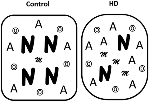
Fig. 2

Illustration of cellular changes during the neurodegenerative process in HD. N neurons; A astrocytes; O oligodendrocytes; M microglia

Another important task relating to the study of human disease biology is the evaluation and selection of model systems that accurately recapitulate the events that take place in the human disease process (Fig. 3). This presents a specific case within the more general issue of comparing and interpreting the extent of similarity between two differential expression profiles. We developed an intuitive and statistically robust strategy to draw such comparisons using a measure that we have termed the “concordance coefficient” (Method 2). Whereas other strategies, such as Gene Set Enrichment Analysis [GSEA; (Subramanian et al. 2005)], have also been applied to the same problem, we feel that our strategy has the advantage of implementing more intuitively interpretable statistics. Another unique feature of our strategy is the consideration of differential expression measures with opposite signs (e.g., increased in one and decreased in the other system), which are subtracted from the overall scoring of association in our method.

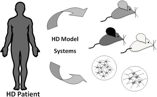
Fig. 3

Illustration of the comparison of disease signatures in model systems to the bona fide human disease. This can be considered as a way to validate model systems for rational selection of models and endpoints to evaluate disease-related mechanisms [see also text and Kuhn et al. 2007]

Both of the following methods are applicable to other data types beyond RNA expression measures: for example, they could also be used to analyze and interpret other high-content molecular data types such as differential proteomic and metabolomic data.

2 Method 1: Application of Population-Specific Expression Analysis (PSEA) to Deconvolve Complex Molecular Profiles into Cellularly Resolved Interpretations of Differential Expression

The characterization of molecular changes in diseased tissues can provide crucial information about pathophysiological mechanisms and is important for the development of targeted drugs and therapies. However, many disease processes are accompanied by changes of cell populations due to cell migration, proliferation, or death (Fig. 2). Identification of key molecular events can thus be overshadowed by confounding changes in tissue composition.

To address the issue of confounding between cell population composition and cellular expression changes, we developed PSEA. This method works by exploiting linear regression modeling of queried expression levels to the abundance of each cell population. Since a direct measure of population size is often unobtainable (e.g., from human clinical or autopsy samples), PSEA instead tracks relative cell population size via levels of mRNAs expressed in a single population only. Thus, a reference measure is constructed for each cell population by averaging expression data for cell type-specific mRNAs derived from the same microarray dataset.

We will illustrate the application of PSEA using the R statistical programming language (R Core Team, http://www.r-project.org) and tools from the Bioconductor project (Gentleman et al. 2004). R/Bioconductor is a natural choice for implementing PSEA as it provides the standard statistical procedures needed for PSEA as well as a convenient and flexible interface for the analysis of genomic data. We explicitly comment every R command so that the code can be more easily understood. In our demonstration, we often provide specific reference to Sect. 2.2 Troubleshooting. This section presents practical advice for each stage of PSEA and describes useful tools for quality and diagnostic checks. It should enable the readers to independently and robustly apply PSEA to their own dataset of interest. The Troubleshooting section can also be read independently of the R code.

Here, we will deconvolve gene expression profiles obtained by microarray analysis of human caudate nucleus samples obtained from HD patients and control subjects (Hodges et al. 2006). The data were obtained using Affymetrix microarrays and are publicly available from Gene Expression Omnibus (GSE3790, http://www.ncbi.nlm.nih.gov/geo/query/acc.cgi?acc=GSE3790). With Affymetrix expression arrays, each transcript is measured by several probes and a summarized expression value is obtained for each probeset. In the following, the term “probeset” thus refers to the expression measurement of a particular mRNA transcript. Except for data preprocessing (Sect. 2.1.2), the demonstration below is not specific to microarray data and can be easily adapted to gene expression profiles obtained with another technology.

First, we will set the stage for the application of PSEA and download raw expression data, process them to obtain gene expression profiles, and prepare population-specific reference signals. We then illustrate the basic principles of PSEA by manually fitting expression models for individual transcripts. Finally, we show how to perform automatic expression model building and deconvolution of entire expression profiles.

2.1 Procedures

We assume that the reader has started an R session on his computer and that the packages GEOquery (Davis and Meltzer 2007), affy (Gautier et al. 2004), annotate (Gentleman), hgu133a.db (Carlson), PSEA (Kuhn 2014), and MASS (Venables and Ripley 2002) are installed. ¹ If in doubt about the meaning of the code, the corresponding help page can be called by typing a question mark followed by the function name, e.g., for the function library():

?library

2.1.1 Loading Required Packages

We start by loading packages needed for downloading data from GEO (GEOquery), processing Affymetrix microarray data (affy), annotating the microarray (annotate and hgu133a.db), for PSEA (PSEA) and a package providing additional useful statistical tools (MASS):

library(GEOquery)

library(affy)

library(annotate)

library(hgu133a.db)

library(PSEA)

library(MASS)

2.1.2 Data Download, Quality Control, and Normalization

We download GEO dataset GSE3790 to the current directory: ² ^, ³

dataset <- getGEO(GEO=”GSE3790″, destdir=”.”)

A GEO dataset generally contains (processed) expression data as well as a lot of project-related information including the sample description. The raw microarray data, however, is available separately. Dataset GSE3790 contains samples from multiple brain regions and HD stages. We will focus on caudate nucleus samples from control subjects and HD grade 1 patients and download the corresponding raw data.

Dataset GSE3790 is comprised of data obtained from two microarray formats (Affymetrix Human Genome U133A and U133B arrays, referred to as GPL96 and GPL97 in GEO, respectively). For simplicity, we will illustrate the work with the U133A microarray format only. We start by extracting the sample information associated with the first microarray: ⁴

information <- pData(phenoData(dataset [[“GSE3790-GPL96_series_matrix.txt.gz”]]))

The sample information includes a phenotypic description of each sample:

phenotypes <- as.character(information[,”characteristics_ch1″])

We identify caudate nucleus samples for control subjects and HD grade 1 patients separately:

control <- grep(“human caudate nucleus control”, phenotypes)

HD <- grep(“human caudate nucleus HD grade 1”, phenotypes)

The sample names for all caudate nucleus control and HD samples can be extracted from the phenotypic description:

control_names <- sapply(strsplit(phenotypes[control], ” “), function(x){x[[1]]})

HD_names <- sapply(strsplit(phenotypes[HD], ” “), function(x){x[[1]]})

Let us keep the samples that passed quality control (QC) as performed in Hodges et al. 2006 (see also Sect. 2.2.1.1). The samples that passed QC are (Supplementary Table 4 in Hodges et al. 2006):

passed_QC <- c (“101”, “11”, “126”, “14”, “15”, “17”, “1”, “20”, “21”, “2”, “52”, “64”, “8”, “H104”, “H109”, “H113”, “H115”, “H117”, “H118”, “H120”, “H121”, “H124”, “H126”, “H128”, “H129”, “H131”, “H132”, “H137”, “H85”, “12”, “13”, “3”, “7”, “HC103”, “HC105”, “HC53”, “HC55”, “HC74”, “HC81”, “HC83”, “HC86”)

We only keep the samples that can be found in the list above:

control <- control[control_names %in% passed_QC]

HD <- HD[HD_names %in% passed_QC]

We can now download the raw data (i.e., Affymetrix .CEL files) corresponding to our selected samples. We first need to look up the corresponding GEO accession IDs:

sample_IDs <- as.character(information[c(control,HD), “geo_accession”])

and we can then get the corresponding raw microarray data files: ⁵ ^, ⁶

datafiles <- sapply(sample_IDs, function(x){rownames(getGEOSuppFiles(x))})

We can finally load the raw data into R

raw_data <- ReadAffy(filenames=datafiles, compress=TRUE)

and normalize it using the RMA method (Irizarry et al. 2003) (see also Sects. 2.2.1.2 and 2.2.1.3):

expression <- 2^exprs(rma(raw_data))

2.1.3 Reference Signals

We previously found that neurons, astrocytes, oligodendrocytes, and microglia were the four cell populations that mostly contributed expression in these caudate nucleus samples [see Sect. 2.2.3 and (Kuhn et al. 2011)]. For each cell population, we then identified several probesets corresponding to mRNAs expressed in that cell type only that can be used to monitor the abundance of the cell population (see Sects. 2.2.2 and 2.2.7.2 Checking dependence on marker genes). For neurons, we selected the following probesets (see Supplementary Table 5 in Kuhn et al. 2011) ⁷ :

neuron_probesets <- list(c(“221805_at”, “221801_x_at”, “221916_at”), “201313_at”, “210040_at”, “205737_at”, “210432_s_at”)

Note that they are assigned to a list where each item can contain one or more probesets measuring expression of the same gene. Here, the first three probesets measure expression of NEFL, and four additional genes are measured by one probeset each. ⁸ The list structure allows us to average expression over probesets measuring the same transcript (for instance, the first three probesets that measure NEFL transcripts) before averaging over several genes. This is what is achieved by the function marker(), resulting in a neuronal “reference signal”:

neuron_reference <- marker(expression, neuron_probesets)

We also define marker probesets and calculate reference signals for the three other cell populations:

astro_probesets <- list(“203540_at”, c(“210068_s_at”, “210906_x_at”), “201667_at”)

astro_reference <- marker(expression, astro_probesets)

oligo_probesets <- list(c(“211836_s_at”, “214650_x_at”), “216617_s_at”, “207659_s_at”, c(“207323_s_at”, “209072_at”))

oligo_reference <- marker(expression, oligo_probesets)

micro_probesets <- list(“204192_at”, “203416_at”)

micro_reference <- marker(expression, micro_probesets)

In addition, we will need a group indicator variable that codes controls as 0 s and HD subjects as 1 s:

groups <- c(rep(0, length(control)), rep(1, length(HD)))

The indicator variable is used to generate an interaction regressor that will allow us to test for differences in cell population-specific expression across groups (HD versus control). For neurons, the interaction regressor is defined as

neuron_difference <- groups * neuron_reference

We create similar interaction regressors for the other three populations:

astro_difference <- groups * astro_reference

oligo_difference <- groups * oligo_reference

micro_difference <- groups * micro_reference

2.1.4 Expression Model for a Single Transcript

We will deconvolve the expression of Calcineurin A (or PPP3CA, measured by probeset 202429_s_at), a gene whose product was previously shown to be decreased in the striatum of HD patients. In PSEA, we use linear regression and model the expression of Calcineurin A in the control samples as a linear combination of the four reference signals:

model1 <- lm(expression[“202429_s_at”,] ~ neuron_reference + astro_reference + oligo_reference + micro_reference, subset=which(groups==0))

The dependence of expression on each reference signal can be visualized as follows (see also Sect. 2.2.5.3):

X11()

par(mfrow=c(1,4), cex=1.2)

crplot(model1, ”neuron_reference”, newplot=FALSE)

crplot(model1, ”astro_reference”, newplot=FALSE)

crplot(model1, ”oligo_reference”, newplot=FALSE)

crplot(model1, ”micro_reference”, newplot=FALSE)

The plots show the strong and specific dependence of Calcineurin A expression on the neuronal reference signal (Fig. 4). The fit summary (an excerpt of which is copied below the command) provides further useful information on the model:

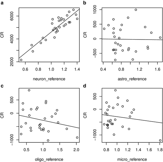
Fig. 4

Component-plus-residual plots showing deconvolved neuronal (a), astrocytic (b), oligodendrocytic (c), and microglial (d) expression of Calcineurin A in control samples

summary(model1)

Output

Coefficients:

Estimate Std. Error t value Pr(>|t|)

Intercept) 103.60 918.19 0.113 0.911

neuron_reference 4604.72 505.05 9.117 2.89e-09 ***

astro_reference −21.35 385.48 -0.055 0.956

oligo_reference −267.37 276.29 -0.968 0.343

micro_reference −288.05 491.12 -0.587 0.563

There is indeed a strong correlation between the expression of Calcineurin A and the neuronal reference signal (neuron_reference), as indicated by the highly significant (p = 2.89e–09) coefficient of this reference signal. This reflects the fact that Calcineurin A is expressed in neurons. The coefficient of the neuronal reference signal (4,605) represents the normalized neuron-specific expression of this gene. ⁹ It is the slope of the regression line in Fig. 4a.

Next, we test for a difference in neuron-specific expression in HD versus control samples and model the expression of Calcineurin A as a combination of the neuronal reference signal and the neuron-specific group difference (neuronal interaction regressor):

model2 <- lm(expression[“202429_s_at”,] ~ neuron_reference + neuron_difference)

The fitted model is visualized as follows:

crplot(model2, “neuron_reference”, g=”neuron_difference”)

It shows that neuronal expression of Calcineurin A is decreased in HD (black squares) compared to control (gray circles) samples, as indicated by the smaller slope of the regression line for HD samples (Fig. 5). The fit summary

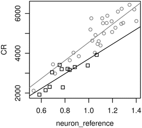
Fig. 5

Component-plus-residual plot showing deconvolved neuron-specific expression in controls (gray circles) and HD subjects (black squares)

summary(model2)

Output

Coefficients:

Estimate Std. Error t value Pr(>|t|)

(Intercept) -387.8 379.6 -1.021 0.313490

neuron_reference 4548.5 345.5 13.165 9.82e-16 ***

neuron_difference −831.5 215.5 -3.859 0.000428 ***

Adjusted R-squared: 0.8898

reveals that the coefficient of the group-specific difference is negative (−831) and highly significant (0.0004). This reflects the fact that Calcineurin A expression is downregulated in neurons of HD patients. Normalized neuron-specific expression in the control group is given by the coefficient of the neuronal reference signal (4,548), and normalized neuron-specific expression in HD is given by the sum of both coefficients (4,548 − 831 = 3,117). These two coefficients are the slopes of the regression lines in Fig. 5. The fold change in neuronal expression can thus be easily calculated using the fitted coefficients:

foldchange <−(model2$coefficients[2] + model2$coefficients[3]) / model2$coefficients[2]

Finally, note that the model fit is excellent (adjusted R ² = 0.89) which means that most of the variations in Calcineurin A expression across samples are explained by the variation in neuronal abundance (as measured by the neuronal reference signal) and the group-specific difference between HD and control samples (see Sect. 2.2.5.4).

2.1.5 Automatic, Stepwise Model Building

An important aspect of PSEA (and statistical model building in general) is how to choose the parameters to include in the model. Indeed, adding more parameters will always result in a better overall fit (and increase the coefficient of determination R ²) but will not necessarily result in a more informative or predictive expression model. The goal thus is to reach a balance between the number of parameters in the model and how much of the data it can account for (see also Sect. 2.2.4).

Several measures have been proposed that can be used as formal criteria to inform model building (also called variable selection). Here, we use AIC [An Information Criterion (Akaike 1974)] to automatically perform model building using a standard stepwise algorithm available in R. The procedure tests the addition of another parameter (or subtraction of an already included parameter) and evaluates the resulting models using AIC. It then chooses the model with the smallest AIC (which represents the best current model) and iterates again until adding or subtracting another parameter does not decrease AIC.

We will deconvolve the expression of AHCYL1 (measured by probeset 200850_s_at) in the control samples. We first define a minimal model containing a constant term only

model3_null <- lm(expression[“200850_s_at”,] ~ 1, subset=which(groups==0))

and use this null model to initiate stepwise model building: ¹⁰

model3 <- stepAIC(model3_null, scope=list(upper=formula(~neuron_reference + astro_reference + oligo_reference + micro_reference), lower=formula(~1)), direction=’both’, trace=0)

Note that the most complex model to consider is specified in the “upper” component of the argument “scope” and contains all four reference signals. The fit summary

summary(model3)

Output

Coefficients:

Estimate Std. Error t value Pr(>|t|)

(Intercept) 1791.0 300.0 5.970 2.29e-06 ***

astro_reference 2253.4 321.6 7.006 1.57e-07 ***

shows that selected model contains the astrocytic reference signal only. This indicates that variations in AHCYL1 expression are strongly correlated with the astrocytic reference signal and that adding any of the other three reference signals does not explain more of the expression variability. In other words, we detected expression of AHCYL1 in astrocytes but not in any of the other three cell populations.

Next, we use a similar model building strategy to deconvolve SEMA6A (measured by probeset 215028_at). In that case, we use both control and HD samples and attempt to detect expression changes. We provide the four reference signals and the four population-specific group differences as possible model parameters:

model4_null <- lm(expression[“215028_at”,] ~ 1)

model4 <- stepAIC(model4_null, scope=list(upper=formula(~neuron_reference + astro_reference + oligo_reference + micro_reference + neuron_difference + astro_difference + oligo_difference + micro_difference), lower=formula(~1)), direction=’both’, trace=0)

summary(model4)

Output

Coefficients:

Estimate Std. Error t value Pr(>|t|)

(Intercept) 19.387 8.450 2.294 0.0274 *

oligo_reference 69.275 8.558 8.094 8.57e-10 ***

oligo_difference 33.264 6.497 5.120 9.13e-06 ***

Adjusted R-squared: 0.8089

The selected expression model thus predicts that SEMA6A is expressed in oligodendrocytes and upregulated in HD.

Automatic model building, however, calls for careful assessment of the selected models. For instance, let us consider the deconvolution of SNC3B (measured by probeset 204722_at):

model5_null <- lm(expression[“204722_at”,] ~ 1)

model5 <- stepAIC(model5_null, scope=list(upper=formula(~neuron_reference + astro_reference + oligo_reference + micro_reference + neuron_difference + astro_difference + oligo_difference + micro_difference), lower=formula(~1)), direction=’both’, trace=0)

summary(model5)

Output

Coefficients:

Estimate Std. Error t value Pr(>|t|)

(Intercept) 407.58 104.60 3.897 0.000383 ***

neuron_reference 744.18 70.55 10.549 7.57e-13 ***

micro_reference −225.13 74.10 -3.038 0.004288 **

Adjusted R-squared: 0.7498

The selected model includes the microglial reference signal, but it is fitted with a significant negative coefficient, and it can thus not be interpreted as an expression model (see Sect. 2.2.5.1). The model suggests, however, that SNC3B mainly has a strong neuronal expression: although the microglial expression was included in the model, it is much less significant. In this case, we could decide to drop the microglial reference (note that the adjusted R ² would not be much different) and settle for an expression model with a single neuronal term.

2.1.6 Deconvolution of Whole Expression Profiles

A stepwise approach to variable selection can be very fast because the search only considers a subset of all possible models. However, it is not guaranteed to find the best model. Moreover, we might want to restrict the statistical models under consideration to those that provide convincing gene expression models (see Sect. 2.2.5.2). In the present case, the small number of samples also makes it unlikely to robustly fit highly complex expression models, and we might want to exclude models containing several parameters coding for expression changes in different cell populations.

The function lmfitst() in the PSEA package efficiently fits a set of models to every transcript in an expression profile and select the best model. We first need to define a model matrix containing all possible parameters as columns (including an intercept as the first column):

model_matrix <- cbind(1, neuron_reference, astro_reference, oligo_reference, micro_reference, neuron_difference, astro_difference, oligo_difference, micro_difference)

We then specify the subset of models that we want to fit ¹¹ as a list. Each list item represents a model by specifying the included parameters (as their column indices in the model matrix). The function em_quantvg() enumerates models automatically:

model_subset <- em_quantvg(c(2,3,4,5), tnv=4, ng=2)

For instance, the 17th model in the list

model_subset[[17]]

Output

1 2 6

Represents an expression model containing an intercept (column 1 in model_matrix), the neuronal reference signal (column 2), and the neuron-specific expression change (column 6).

We can then fit each probeset in the expression profile with all models in the subset, and for each probeset, select the best expression model (using AIC as a criterion):

models <- lmfitst(t(expression), model_matrix, model_subset, lm=TRUE)

The function lmfitst() returns two lists. The first contains the identity of the best and next best models for each transcript (see also Sect. 2.2.7.1). The second contains details of the (fitted) best model for each transcript. For PPP3CA, for instance, the selected expression model contains the parameters corresponding to neuronal expression and neuron-specific expression change (as we manually worked out in Sect. 2.1.4):

summary(models[[2]][[“202429_s_at”]])

Only gold members can continue reading. Log In or Register to continue