Genomics

Fig. 4.1

DNA–chromatin complexes a binding of basic histone proteins, b a nucleosome—two turns of DNA wrapped around core histones, c electron micrograph of nucleosomal filaments, d cross section of a chromatin fibre. From Strachan and Read (2011)

The tightness of these complexes is one of the key factors determining whether genes can be transcribed to RNA (turned on); the tighter the complexes are, the less likely the transcription of genes contained in the compacted segment of DNA (Fig. 4.2). During cell division, the entire chromosomes are tightly bundled up to facilitate their sorting into the daughter cells; no genes are transcribed in this phase of the cell cycle (Fig. 4.2, far right). The highly condensed form of chromatin is called heterochromatin, while the uncondensed form is euchromatin (Text Box 4.1). The uncoiled molecule of DNA present in euchromatin is ready for the synthesis of new DNA (replication) and RNA (transcription).

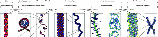
Fig. 4.2

Three levels of chromatin organization: (1) DNA wraps around histone proteins forming nucleosomes that look like beads on a DNA string; this is when genes can be transcribed (turned on); (2) multiple histones wrap into a 30 nm fibre consisting of nucleosome arrays in their most compact form; this is when genes in this segment of DNA are “turned off”; and (3) higher-level DNA packaging of the 30 nm fibre into the metaphase chromosome during cell division; this is when all genes are “turned off”. From http://www.answers.com/topic/chromatin

As the brain and body grow during development and old cells are replaced in adulthood, new somatic cells (all diploid) are generated through a typical form of cell division: mitosis. In the S phase of the cell cycle, DNA is replicated and the cell now contains a double amount of DNA (~14 pg); each of the 46 chromosomes now has its own homologue. These “old” and “new” chromosomes, tied together at a centromere, are referred to as “sister chromatids”. In the M phase of the cycle, sister chromatids are separated—yielding a total of 92 chromosomes (i.e. four 23-chromosome sets) that are subsequently distributed into two daughter cells (46 chromosomes in each cell). It has been estimated that, over the course of the human lifespan, about 10¹⁷ mitotic cell divisions take place (Strachan and Read 2011, p. 32).

In the case of germ-line (diploid) spermatocytes and oocytes, new cells are generated through reduction division, meiosis, which produces haploid gametes (sperm and eggs; see Text Box 4.2).

Text Box 4.2. Production of haploid gametes: Meiosis

Meiosis progresses differently in the spermatocytes and the oocytes. For the spermatocytes, the first phase of meiosis (meiosis I) involves symmetric division of the (diploid) primary spermatocytes, resulting in two (diploid) secondary spermatocytes. In the second phase (meiosis II), another round of the symmetric cell division proceeds without DNA replication and generates two haploid spermatids per secondary spermatocyte. For the oocytes, meiosis I involves an asymmetric division that produces one diploid secondary oocyte and one polar body (which is discarded). In meiosis II, another asymmetric cell division, this time without DNA replication, produces one haploid mature egg (and one polar body, also discarded).

The meeting of an egg and a sperm represents a key event in the generation of genetic diversity through (1) an independent assortment of the maternal and paternal chromosomes, and (2) recombination.

Fertilization of a haploid egg by a haploid sperm results in a diploid zygote containing two sets of chromosomes—maternal and paternal. During meiosis I, the maternal and paternal homologues come together, forming the bivalent. After DNA replication, each of the homologous chromosomes of a given bivalent consists of two chromatids,¹ for a total of four strands of DNA. Next, the mitotic spindles pull one complete chromosome (i.e. two chromatids joined at centromere) towards each pole, which of the 23 chromosomes to go to which pole is random. Therefore, each daughter cell produced during the final phase of cell division inherits a random (independent) assortment of the maternal and paternal chromosomes (e.g. chromosomes 1, 4–6, 10, 12–14, 16, 17, 22, 23 and X from the mother, and chromosomes 2, 3, 7–9, 11, 15, 18–21 and X from the father). Given the number of chromosomes in one set (23), there are about 8,000,000 (2²³) possible combinations of the maternal and paternal chromosomes in the gametes (per meiosis; Strachan and Read 2011, p. 34).

The other key event occurring during meiosis is that of recombination (Fig. 4.3). As mentioned above, the duplicated maternal and paternal homologues form a bivalent consisting of four chromatids. Recombination (or crossover) occurs through a physical breakage at a corresponding location on two of the four strands, one maternal and one paternal, and the subsequent rejoining of the crossed-over fragments of the chromosomes. The recombined homologues remain connected at the point of a crossover, the chiasma, which is severed only when the mitotic spindles start pulling the chromosomes towards the poles. There are ~55 chiasmata per cell during the male meiosis (but 50 % more during the female meiosis), thus indicating the frequency of recombination during sexual reproduction (Strachan and Read 2011, p. 35).

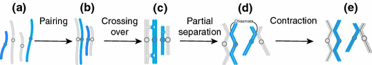
Fig. 4.3

Meiosis: an example of two chromosomes from the mother (light blue) and the father (dark blue) a Chromosomes are duplicated (chromatids) but remain unpaired, b duplicated homologues of the maternal and paternal chromosome (two chromatids each) pair up to form a bivalent (four chromatids), c recombination (crossing over): physical breakage and subsequent rejoining of maternal and paternal chromosome fragment (in this example, there are two crossovers in the bivalent on the left side and one in the bivalent on the right), d homologous chromosomes separate slightly, except at the chiasmata (points of crossover), and e bivalents contract and transit to metaphase. From Strachan and Read (2011)

Together, the two mechanisms of combining maternal and paternal genetic material represent a major source of genetic variability in the human population; one ensuring a combination of genes located on different chromosomes (chromosomal assortment) and the other mixing maternal and paternal genes within a chromosome (recombination).

4.2 Genetic Code, Gene Transcription and Translation

Let us now focus on the actual DNA molecule and talk about the genetic code.

The DNA molecule is a double helix in which two (complementary) strands of DNA are bound to each other through nitrogenous bases (base pairs). In DNA, the bases are adenine (A), cytosine (C), guanine (G) and thymine (T); the canonical (Watson–Crick) base pairings are A–T and G–C (Watson and Crick 1953). The backbone of each strand is made of a five-carbon sugar (deoxyribose) linked to the next sugar with a phosphate (see Figs. 4.4 and 1.2).

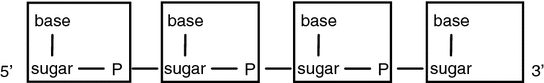
Fig. 4.4

Two building blocks of a DNA molecule: a base (A, C, G or T) and a sugar (deoxyribose) linked to the next sugar by a phosphate (P). Each nucleotide (indicated by a rectangle) consists of a base, a sugar and a phosphate. The 5′ (five prime) and 3′ (three prime) ends refer, respectively, to the 5th and 3rd carbon in the sugar. Modified from Strachan and Read (2011)

Nucleotides are the basic DNA units; each nucleotide consists of a base, a sugar and a phosphate. The genetic code consists of nucleotide triplets (e.g. ATG) that are transcribed to messenger RNA (mRNA) as three-letter codons. In mRNA, each of 64 possible codons corresponds to one of 20 amino acids and to one of three so-called STOP codons. One codon (AUG) codes an amino acid (methionine) and also indicates where translation into a protein begins (START codon). Table 4.1 contains a DNA codon table, indicating DNA bases on the “sense” DNA strand (see below).

Table 4.1

DNA codon table

Genetic code
1st base	2nd base								3rd base
1st base	T		C		A		G		3rd base
T	TTT	(Phe/F) Phenylalanine	TCT	(Ser/S) Serine	TAT	(Tyr/Y) Tyrosine	TGT	(Cys/C) Cysteine	T
	TTC	(Phe/F) Phenylalanine	TCC		TAC	(Tyr/Y) Tyrosine	TGC	(Cys/C) Cysteine	C
	TTA	(Leu/L) Leucine	TCA		TAA	Stop	TGA	Stop	A
	TTG		TCG		TAG	Stop	TGG	(Trp/W) Tryptophan	G
C	CTT		CCT	(Pro/P) Proline	CAT	(His/H) Histidine	CGT	(Arg/R) Arginine	T
	CTC		CCC		CAC	(His/H) Histidine	CGC		C
	CTA		CCA		CAA	(Gln/Q) Glutamine	CGA		A
	CTG		CCG		CAG	(Gln/Q) Glutamine	CGG		G
A	ATT	(Ile/I) Isoleucine	ACT	(Thr/T) Threonine	AAT	(Asn/N) Asparagine	AGT	(Ser/S) Serine	T
	ATC		ACC		AAC	(Asn/N) Asparagine	AGC	(Ser/S) Serine	C
	ATA		ACA		AAA	(Lys/K) Lysine	AGA	(Arg/R) Arginine	A
	ATG^[A]	(Met/M) Methionine	ACG		AAG	(Lys/K) Lysine	AGG	(Arg/R) Arginine	G
G	GTT	(Val/V) Valine	GCT	(Ala/A) Alanine	GAT	(Asp/D) Aspartic acid	GGT	(Gly/G) Glycine	T
	GTC		GCC		GAC	(Asp/D) Aspartic acid	GGC		C
	GTA		GCA		GAA	(Glu/E) Glutamic acid	GGA		A
	GTG		GCG		GAG	(Glu/E) Glutamic acid	GGG		G

The DNA codons occur on the sense DNA strand and are arranged in a 5′ → 3′ direction

Clearly, the genetic code must be read in the correct direction. During the synthesis of both the new DNA (replication) and RNA (transcription), the DNA and RNA polymerases copy the code of the template strand of DNA in the 5′ → 3′ direction; the 5′ and 3′ ends have sugar residues in which carbons number 5 and 3, respectively, are not linked to another sugar. The nucleotide sequence of RNA transcript (mRNA) is complementary to the template (sense) strand of DNA and, as such, it is identical to the sequence of the non-template (anti-sense) strand (with one exception: thymine is replaced by uracil).

All cells in the body contain the same DNA. Whether a particular cell synthesizes proteins that turn it, for example, into a pyramidal neuron or a Chandelier interneuron depends mainly on which of its genes are transcribed into messenger RNA. Gene transcription is regulated by transcription factors, a family of proteins that bind to a particular DNA sequence elements—a promotor—located upstream² from a gene and in its immediate vicinity. Once bound to a promotor,³ a transcription factor guides the RNA polymerases transcribing the template strand of DNA into RNA. In addition to promotors, transcriptional activity can be enhanced or inhibited by “enhancers” or “silencers”, respectively, as well as by a number of epigenetic mechanisms (see Chap. 5). Once a full RNA transcript is synthesized, a set of steps ensues that it makes a “mature mRNA”. One of the key steps in this chain of reactions is RNA splicing, whereby the non-coding parts of the gene (introns) are removed and the remaining coding sequences (exons) are tied together to form a shorter mRNA (Text Box 4.3).

Text Box 4.3. Exons and introns

An exon (a DNA region that will be expressed) is part of DNA that is transcribed to mRNA and, in most cases, translated into a protein. An intron (intragenic region) refers to a DNA sequence within a gene that is removed (by splicing) during transcription and, therefore, is not the part of the final mRNA. Typically, an intron is recognized by the fact that it starts with a GT and ends with an AG (the GT–AG rule). For the majority of multi-exon human genes (Pan et al. 2008), this process may bring together a slightly different subset of exons. Such an “alternative splicing” may result, after translation, in different forms of the same protein.

The final step on the road from DNA to protein is translation. Unlike the preceding steps, which all take place in the cell nucleus, translation occurs on ribosomes, located in the cell cytoplasm (Fig. 1.2). This is where the genetic code is translated into a polypeptide: an RNA codon into an amino acid. As we see in Table 4.1, most amino acids are coded by more than one codon, hence, “degeneracy” of the genetic code. Translation results in a chain of amino acids—a polypeptide—that is often modified (during or after translation) by other chemical processes, such as phosphorylation, methylation or acetylation. The final product—a protein—consists of one or more polypeptides, which may undergo further post-translational modifications, co-determining the ultimate structure (and hence, functionality) of the protein.

Overall, given the above rules governing replication and transcription of DNA, it is not surprising that one letter of the genetic code can make a big difference in the final outcome: the amount and structure (and therefore function) of a protein.

4.3 DNA Variations

Variations in DNA inherited through the germ line from our parents represent the main molecular mechanism underlying the heritable portion of inter-individual variability in brain and behaviour. In general, one can distinguish between (1) single–nucleotide variations, which involve base substitutions, deletions and insertions of a single nucleotide; and (2) multiple–nucleotide variations, which include insertions and deletions (so-called indels) of multiple nucleotides, as well as copy-number variations (CNVs) and inversions. In current genetic mapping studies (see Sect. 4.4), the most commonly employed DNA variations are single-nucleotide polymorphisms (SNPs) and CNVs.

SNPs are variations in the nitrogenous base of a single nucleotide (e.g. A instead of G) located anywhere in the DNA sequence. It has been estimated that any two individuals would differ, on average, in one out of 1,200 bases; with three billion bases per 23 chromosomes, this represents about 2,500,000 SNPs distinguishing any two individuals (http://hapmap.ncbi.nlm.nih.gov). About 10 million “common” DNA variants (primarily SNPs) occur with a frequency higher than 1 % across various human populations, as sampled by the Human Genome Project, the SNP Consortium and the International HapMap Project (The International HapMap 3 Consortium 2010). The latest version of the SNP database (dbSNP Build 135, human Genome Build 37.3; http://www.ncbi.nlm.nih.gov/SNP/) contains a total of 41,740,143 validated SNPs (reference SNP [rs] ID numbers), of which about 22 million are located within and/or near genes⁴ and about 19 million are found in intergenic regions.

When located in exons (~3 million out of all 41 million SNPs), a SNP can be either non-synonymous or synonymous; the former refers to the fact that the sequence substitution results in a different amino acid, whereas this is not the case for the latter (recall the “degeneracy” of the genetic code, see Table 4.1). For example, the change of “G” to “A” in the first letter of a DNA codon for valine (GTG) results in a codon that codes instead for methionine (ATG; see Table 4.1). This kind of genetic variation is found, for example, in a commonly studied SNP (rs6265) of the BDNF gene (Text Box 4.4).

Text Box 4.4. A non-synonymous SNP in the BDNF gene

A commonly studied SNP (rs6265) in BDNF—the “G196A” DNA polymorphism—results in a “val66met” (valine to methionine) polymorphism in the proBDNF polypeptide. The number between G and A refers to the position of the nucleotide in cDNA, and the number between val and met refers to the position of the amino acid in the polypeptide/protein. This polymorphism appears to affect intracellular packaging of proBDNF, its axonal transport and, in turn, activity-dependent secretion of BDNF at the synapse (Chen et al. 2004).

Although it is more likely for the non-synonymous SNPs to influence the ultimate function of a given gene product, this is also possible for the synonymous SNPs and SNPs located in introns or intergenic regions. Even though synonymous SNPs do not change amino acids, they may affect the function by influencing, say, gene expression. The distinction between “functional polymorphisms” and “markers” will be discussed in the next Sect. 4.3.

CNVs refer to various quantitative variations in the genome, including tandem repeats, deletions and duplications; they can vary in size between ~1 kb and 1 Mb (Text Box 4.5).

Text Box 4.5. Variable Number of Tandem Repeats (VNTR)

VNTR is an example of a CNV commonly used in genetic studies. Historically, VNTRs were used in the first genome-wide studies of complex traits. Some of VNTRs are functional polymorphisms; for example, we use the variable number of CAG triplets in Exon 1 of the androgen receptor gene in this context (see Fig. 9.4).

In a survey of CNVs larger than 500 bp, about 8,000 different CNVs were revealed in DNA from 40 individuals. As shown in Fig. 4.5, the majority of these genetic variations were found in intergenic regions (Conrad et al. 2010), where they might influence expression of the genes located in their vicinity. For example, many developmental genes are flanked by large intergenic regions (gene deserts) containing enhancers of gene expression (Klopocki and Mundlos 2011). CNVs might be behind some of the associations previously observed between SNPs and complex traits: almost a third of SNPs associated with a complex trait are in LD with a CNV (Conrad et al. 2010). This opens up the possibility that such SNPs mark the locations of “causal” CNVs.

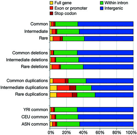
Fig. 4.5

Copy-number variations. Population frequency classes: common (MAF > = 0.1), intermediate (0.1 > MAF > 0.01) and rare (MAF < = 0.01). YRI, Yoruba from Ibadan, Nigeria; CEU, Utah residents with ancestry from northern to western Europe; ASN, denotes JPT (individuals in Tokyo, Japan) and CHB (individuals in Beijing, China). From Conrad et al. (2010)

To appreciate how a person’s genome might differ from the “average” genome, we can compare the full DNA sequence of an individual with a reference assembly.⁵ This has been done for the founder of Celera (https://www.celera.com), Craig Venter’s own DNA sequence. Venter’s genome differs from the reference assembly in the following features: 3.2 million SNPs; 292,000 heterozygous insertion/deletion variants (indels); 559,000 homozygous indels; 90 large inversions; and 62 large copy-number variants. Almost 44 % of Venter’s genes had a sequence variant, with 17 % of them encoding an altered protein (Levy et al. 2007). This level of knowledge of the human genome represents an extraordinary platform from which to embark on mapping genotype-phenotype associations.

Only gold members can continue reading. Log In or Register to continue