Microelectrode Signal Analysis Techniques for Improved Localization

Microelectrode Signal Analysis Techniques for Improved Localization

JAMES MCNAMES

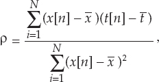
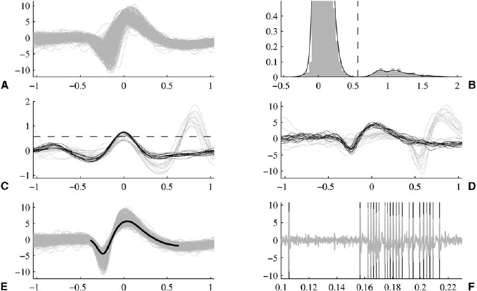
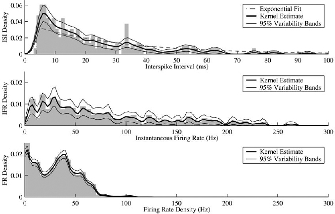
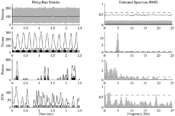
This chapter reviews some of the most popular methods of extracellular neuronal signal analysis. Although these techniques are generally applicable to most extracellular neuronal activity the discussion is focused on the analysis of microelectrode recordings for the purpose of identifying structures near the globus pallidus internus (GPi) and subthalamic nucleus. These are popular targets for ablation or placement of deep brain stimulator electrodes in stereotactic neurosurgery for patients with Parkinson’s disease. All of the methods discussed in this chapter have been used for off-line analysis of microelectrode recording (MER) signals, and some of these methods are included in modern computer-based microelectrode recording and analysis systems.

Signal Acquisition and Preconditioning

Prior to MER signal analysis, the continuous-time voltage signal is amplified by a preamplifier located near the electrode to reduce electrical noise. The preamplifier gain typically ranges from 5000 to 10,000. Prior to sampling, the signal is filtered to remove drift, to further reduce noise, and to prevent aliasing. The filter is usually a bandpass filter with a passband range of 300 to 10,000 Hz. After these preconditioning steps, the signal is sampled with an analog-to-digital converter with a sampling rate of at least 24 kHz. To prevent distortion due to aliasing, the sample rate should be significantly greater than twice the highest passband frequency of the filter. The digitized signal can then be analyzed with discrete-time processing methods in nearly real time and permanently stored on electronic media. Some groups use analog electronics equipment for on-line analysis and do not digitize the MER signals.

Spike Discrimination

Because each action potential represents a binary all-or–none event, the majority of MER signal analysis has been applied to the time sequence of action potentials recorded from single units (i.e., neurons). This binary-valued time series is called a spike train. The purpose of spike discrimination is to identify the times of either the action potentials with the largest amplitude from a single neuron or the action potentials from multiple neurons that can be consistently detected. In the latter case, the action potentials from different neurons must be distinguished. Methods for doing this are discussed in the following section.

The simplest and most common method of spike discrimination is threshold detection.1 For this form of detection, every point in time at which the signal exceeds a user-specified limit is labeled as an action potential. One of the advantages of this method is that it may be implemented on analog oscilloscopes without the need for sampling and discrete-time analysis. The disadvantage of this method is that it is not always possible to set a threshold to isolate a single unit or all of the units of interest.

Many investigators use more elaborate analog window discriminators. These are designed to generate a timing pulse corresponding to action potentials if the signal rises above a lower threshold without exceeding an upper threshold as it falls below the lower threshold. More advanced discriminators generate timing pulses if the signal falls below the lower threshold within a specified amount of time. This feature enables users to separate action potentials of similar amplitude and different duration. Window discriminators enable more accurate discrimination than simple thresholds but require more tuning and user skill.

More elaborate methods of spike discrimination are possible with discrete-time processing methods. Some of the more advanced algorithms search for large first derivatives in the signal after low-pass filtering.2–4 Action potentials are labeled at points where the derivative is larger than a user-specified threshold.

One of the most accurate methods of spike discrimination is template pmatching.^5–8 This method compares shifted versions of the signal with a short segment representing a prototypical action potential. The template may be from a fixed library or estimated from the MER signal. A measure of similarity between the template and a segment of the MER signal is used to determine whether the segment contains an action potential. The most common measure of similarity is the mean squared error (MSE).

We use a three-stage process for spike discrimination. During the first stage, the fourth moment of the signal is low-pass filtered, and the density of peaks is estimated to find no more than four modes. An initial threshold is selected automatically as the minimum between the largest mode and the second largest mode in the density. All of the peaks above this threshold are used as the first estimate of the action potential locations. The second stage takes the median of all the initial action potentials as a first estimate of the template. The template is compared with the signal to find the points with the smallest MSE. An estimate of the MSE minimal density is constructed, and all of the points in the smallest mode are used as a second estimate of the action potential times. This process is repeated three times to find the final template. In the final stage, the template is compared with the signal to find the points of maximum correlation. A density estimate is used to identify the largest mode and set a final threshold to distinguish correlation peaks corresponding to action potentials and those representing noise (see Fig. 13–1). To ensure action potentials that have a significantly larger amplitude than the template are included, we use a modified coefficient of correlation,

where x[n] is the signal segment being compared with the template, t[n], and and are the sample averages of the signal segment and the template, respectively. This coefficient of correlation can have values larger than 1 if x[n] is similar to t[n] but larger in amplitude. Figure 13–1 shows a series of plots from different stages of the algorithm applied to a bursting globus pallidus externus cell. In this case, the action potentials decrease in amplitude during bursts, causing significant variation in the action potential amplitude. Despite this variation, this algorithm was able to discriminate the action potentials accurately.

Spike Sorting

Common surgical practice for subthalamic nucleus and GPi targeting is to seek only well-isolated units.9 It is unknown whether the discharge patterns of well-isolated units with large action potentials are representative of the activity within the region. Few MER investigators have analyzed multiunit signals due to the complexity of distinguishing action potentials of different units. This problem is known as spike sorting, and many algorithms have been developed for this task. Most of these algorithms require that all of the spikes be detected (without discrimination) prior to sorting.

One of the most difficult problems for spike-sorting algorithms is identifying and separating action potentials that overlap in time. Several investigators have demonstrated that the failure to identify spikes from multiple neurons when they overlap can distort the cross-correlation functions of cell pairs and the autocorrelation functions of individual cells.^8,10

A detailed review of spike-sorting algorithms is beyond the scope of this chapter. The interested reader is referred to the review by Lewicki¹ and some of the recent articles on this topic.^7,11–15

Single-Unit Spike Train Analysis

Although many surgeons use analog window discriminators, oscilloscopes, and audio speakers for online MER analysis and physiological localization during surgery, considerable progress has been made in developing useful off-line discrete-time analysis tools. This section reviews some of the most common methods of analyzing single-unit spike trains.

Histograms

Histograms are a common tool to estimate the distribution of intervals and estimated firing rates of a spike train. The interspike interval histogram is one of the most popular among these and estimates the distribution of intervals between each pair of spikes. The user must specify the length of the segment analyzed, the bin width, and the range of the histogram. Typical values are 0.1 to 5.0 msec bin widths displayed over ranges of 90 to 500 msec calculated from segments lasting 0.5 to 30 sec.16–18 The instantaneous firing rate (IFR) is defined as the inverse of the ISI. The IFR histogram is useful to estimate the distribution of neuronal firing rates, although this estimate can be misleading because it underestimates the occurrence of low firing rates and overestimates the occurrence of large firing rates.

Figure 13–1 Example of spike discrimination based on a generalized coefficient of correlation (ρ). (A). Overlapping action potentials detected from the first stage of the algorithm. (B). Histogram of peaks in ρ and threshold for discriminating action potentials from noise (dashed vertical line). (C). Overlap plot of ρ for the 15 worst detected (black) and 15 best undetected (gray) action potentials. (D). Overlap plot of the 15 worst detected (black) and 15 best undetected (gray) action potentials. (E). Overlap plot of all detected action potentials (gray) and the template (black) used to generate them. (F). Example of detected action potentials (black vertical lines) during a burst with decreasing amplitude.

More advanced methods of statistically estimating distributions have not been widely applied. For example, kernel density estimators are a popular method of creating a continuous nonparametric estimate of an unknown probability distribution function (PDF).19,20 If a gaussian kernel is used, the estimated density can be written as

where x[i] is the ith data point and σ is a user-defined parameter that controls the smoothness of the estimate. The variability of this estimate is usually measured by bootstrapping techniques. This is done by repeatedly creating density estimates using synthetic datasets created by resampling the original dataset with its replacement. This process is repeated many times, 200 to 2000, and a user-specified percentile of the range of density estimates is plotted to demonstrate the variability of the estimate. These bands are not confidence intervals, but they provide the user with an idea of how variable the estimator is. Figure 13–2 shows typical ISI and IFR histograms, kernel density estimates of the distributions, and variability bands for a 10 sec recording of a subthalamic nucleus cell.

Mehta and Bergman described an alternative procedure for estimating the confidence interval of the histograms based on the assumption that the ISI follows a Poisson distribution.¹⁷ The confidence intervals are inaccurate when the underlying distribution is not Poisson.

If the spike train could be modeled as a Poisson process in which the spikes occur at random instants of time at an average rate of λ, the interspike intervals should have an exponential distribution.²¹ A more accurate model of the process would take into account the refractory period that effectively sets a lower limit on the interspike intervals. This could be achieved by modeling the truncated interspike intervals, defined as the measured interspike intervals minus the refractory period, with an exponential distribution. The spike train is then modeled as a modified Poisson process with dead time. The refractory period can be estimated as the minimum ISI observed. Figure 13–2 shows an example of the estimated exponential distribution with the maximum likelihood estimate of the distribution parameter.

Figure 13–2 Interspike interval (ISI), instantaneous firing rate (IFR), and firing rate density (FRD) histograms from a 10 sec recording of a subthalamic nucleus cell. The ISI histogram was constructed with 1 msec bin widths, and the firing rate histograms were constructed with 5 Hz bin widths. The variability bands of both histograms were created by bootstrapping with 1000 resampled datasets. The kernel estimate of the density is also shown, with kernel widths of 1.5 msec for the ISI and 2.5 Hz for the firing rate histograms. The ISI plot also shows the maximum likelihood fit of an exponential distribution, with an estimated dead time of 3.8 msec. The histograms are scaled to have unit area.

The exponential random variable is the only random variable with the memoryless property:

where P[δ > h] is the probability that the interspike interval δ is greater than time h. Thus, if a sample distribution of ISIs is significantly different than the exponential distribution, we can conclude that the spikes do not occur independently of one another and time series analysis of the spike train is warranted. A statistical hypothesis test, such as the nonparametric Kolmogorov-Smirnov or Lilliefors test, can be used to determine if a truncated sample of ISIs is significantly different than an exponential distribution.22 For the example shown in Figure 13–2, the null hypothesis was rejected at a significance level of .05 (p < 0.0001). Bursting and pausing are examples of common phenomena observed in MER targeting of GPi and subthalamic nuclei that cannot be accurately modeled as a Poisson process with dead time.

Firing Rate Density

The discharge pattern of a spike train can be visualized by smoothing the estimated firing rate.17,23 This is done by filtering the spike train with a low-pass filter that has unity gain at 0 Hz. It is preferable to use a finite impulse response (FIR) filter with nonnegative coefficients to prevent ringing at abrupt edges that is common to low-pass filters. An example of such a filter is the weighted moving average filter

where ω(k) are the window coefficients. There are many reasonable choices for the window function, including the raised cosine, rectangular, Bartlett (triangular) Hanning, Hamming, and Blackman windows.²⁴ The Blackman window,

is a good choice. To ensure the window has unity gain at 0 Hz and to convert the density from units of spikes per sample to spikes per second, it is necessary to normalize the window,

where f_s is the sample rate of the spike train. Figure 13–3 shows an example of the firing rate density of a simulated Poisson process, a GPi cell with tremor, a bursting GPe cell, and a subthalamic nucleus cell.