Neuroimaging Methods in the Study of Childhood Psychiatric Disorders

The MRI Unit at Columbia University and New York State Psychiatric Institute

Abbreviations

Anterior Commissure

ADHD

Attention-Deficit/Hyperactivity Disorder

BOLD

Blood Oxygen Level Dependent

CSF

Cerebrospinal Fluid

Computed Tomography

DTI

Diffusion Tensor Imaging

Diffusion-Weighted

EEG

Electroencephalography

fMRI

Functional Magnetic Resonance Imaging

GABA

γ aminobutyric acid

FOV

Field of view

ICA

Independent component analysis

Ins

Myo-inositol

ISI

Inter-Stimulus interval

MEG

Magnetoencephalography

MRI

Magnetic Resonance Imaging

MRS

Magnetic Resonance Spectroscopy

NAA

N-acetyl aspartate

Posterior Commissure

PET

Positron Emission Tomography

PPM

Parts per Million

ROI

Region of Interest

SNR

Signal-to-Noise Ratio

SPECT

Single Photon Emission Computer Tomography

Tesla

tCh

Total Choline

tCr

Total Creatine

Tourette Syndrome

Overview

The direct observation of the structural and functional organization of the brain using neuroimaging methodologies is playing an increasingly important role in the study of childhood psychiatric disorders. Ultimately, this improved understanding of the causes of psychiatric disturbances in children will suggest new and more specific treatments for these conditions, including the means for planning individualized treatments and for monitoring therapeutic response.

We aim to provide herein a comprehensive introduction to neuroimaging methods that will help readers to become informed consumers of such research. In particular, our goal is to describe the advantages and limitations of each technology that must be appreciated when gauging the merits of an imaging study. We will also provide brief examples of the implementation of these techniques to the study of childhood psychopathologies and the kinds of insight into pathophysiology that they can provide.

We will review a range of existing and emerging technologies that are useful in neuroimaging studies of normal and abnormal brain development, focusing in particular on magnetic resonance imaging (MRI) because of its relative safety and widespread use compared with other imaging methods. We will discuss only briefly the principles of positron emission tomography (PET) and single photon emission computer tomography (SPECT) because these require the administration of radioactive tracers. Although some investigators have argued persuasively that the degree of radiation exposure (often less than the equivalent of a chest x-ray) poses no significant risk to children (1,2), these methods are unlikely to find widespread acceptance in research protocols, particularly in those that include healthy control children. MRI will therefore almost certainly continue to be the most widely used imaging modality for the study of children. We will also briefly review electroencephalography (EEG) and magnetoencephalography (MEG), given their increasing use in the study of brain function in children.

What Is an Image?

The basic unit of a two-dimensional digital image is a picture element or “pixel.” A pixel is a two-dimensional square that has a single level of grayness ranging from black to white. Each pixel represents a corresponding three-dimensional cube of tissue in the brain called a volume element or “voxel.” Many pixels assembled into a larger square or rectangular array constitute an image that represents a corresponding three-dimensional “slice” of brain tissue. Each pixel of the image has associated with it a number that represents some feature of the corresponding voxel in the brain. This feature may be, for example, the degree of x-ray attenuation or tissue density (in x-ray and computed tomography, CT), the magnitude of reflected sound waves from soft tissue interfaces within the body (by ultrasound, US), the concentration of photons emitted by the radioisotopes delivered to a specific tissue or chemical receptor within the patient’s body (PET and SPECT), the number of protons in the tissue (in anatomical MRI), the relative concentration of deoxyhemoglobin (in functional MRI or fMRI), or the concentration of a chemical compound (in magnetic resonance spectroscopy or MRS). This physical characteristic of the tissue is encoded within a signal coming from the brain. In a gray-scale image, the number associated with a pixel, and therefore the physical feature of the brain that it represents, is assigned a level of grayness ranging from black to white. The strength of the signal coming from a single voxel, and therefore the level of grayness of its corresponding pixel, will differ between neighboring voxels if the average physical or chemical features of those voxels differ. The differing levels of grayness across an image thus represent differences in the physical property (e.g., density, water content, protons, deoxyhemoglobin, or chemical compounds) of the brain as measured by a particular imaging modality.

The quality of an image depends on the characteristics of the signal within and across pixels, which include resolution, signal-to-noise ratio, and contrast. Resolution refers to the size of the voxels from which a radio signal is being measured. The smaller the voxels, the better the resolution. Higher resolution allows for greater discrimination of neighboring structures within the brain (Figure 2.4.1.2). At a lower resolution, two differing structures may be included within the same voxel; the signal that originates within each of the two structures will be averaged into a single signal (called a partial volume effect). The pixel representing this averaged signal will be assigned a single level of grayness.

As with any measurement process, repeated measures of the physical properties of a voxel in the brain will have some degree of error that centers around an average value. Random error, or noise, in the measurement of signal within each voxel degrades the quality of the image. The ratio of the strength of the signal to the noise of the signal within each pixel provides a useful index of image quality. Whenever signal strength decreases, or when noise increases, the signal-to-noise ratio (SNR) decreases and image quality degrades (Figure 2.4.1.1). For example, in MRI, the strength of the magnetic field, a primary determinant of SNR, is measured in Tesla (T), a unit of measurement that represents the number of magnetized water molecules within a specific volume of tissue. With a magnetic field of a higher strength, the number of hydrogen protons excited within magnetized water molecules is greater. This in turn increases the strength of the signal coming from any given voxel, thus improving the quality of the image.

On any MRI scanner, a common way to improve SNR is to increase the size of voxels, thereby increasing the volume of brain tissue that provides the radio signal for each pixel. Voxel size can be increased by increasing slice thickness or by increasing the dimensions of the voxels in the imaging plane, which in turn is achieved by decreasing the number of voxels into which an image is divided (termed the “matrix” of the image). The field of view (FOV) of the image (the height and width of the two-dimensional slice of brain tissue being imaged), is approximately 25 cm × 25 cm in a human. In a typical image from MRI, this FOV is broken into 256 segments, or matrixes, in each direction. Therefore, the matrix size for the 2D slice is said to be 256 × 256, making each voxel slightly smaller than 1 mm × 1 mm in size within the slice of the brain being imaged (250 mm broken into 256 segments yields individual segments of 250/256 = 0.98 mm in length for each of the two dimensions of the FOV). Thus, in order to increase the voxel size and subsequently the SNR, one must either increase the FOV or decrease the matrix size,
both of which will decrease the spatial resolution of the image. Conversely, increasing the resolution in an MR image will typically decrease the SNR.

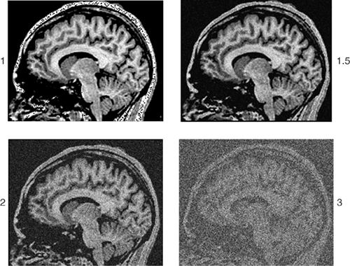FIGURE 2.4.1.1. Signal-to-noise ratio. The noise of a single cross-sectional sagittal view of the brain is varied from the original image (upper left) to a value that is: 1.5 times larger (upper right), 2 times larger (lower left), or 3 times larger (lower right). Increasing the noise three-fold makes this particular image barely discernible.

Finally, image contrast refers to the difference in the strength of signal acquired from adjacent tissues. The level of contrast reflects how well signals that originate in voxels of differing tissue types in the brain are discriminated, as reflected by the differing levels of grayness across the pixels of the image. Recall that the range of biological information acquired during the scanning process is recast in terms of gray scale in order to generate a 2D black and white image. By convention, most such MR images are assigned gray-scale values ranging from 0 (pure black) to 255 (pure white). Pixels with no relative contrast would all be assigned a single value and therefore would appear as uniformly black, white, or gray in an image. Pixels with maximum contrast would receive a gray-scale value of either 0 (black) or 255 (white), with no intervening values (Figure 2.4.1.2). An image with optimal contrast would assign the most widely differing gray-scale values to voxels whose signal strengths may differ only slightly, but in a way crucial for the investigative purposes of the scan. For example, to distinguish gray from white matter optimally, gray-scale values would discriminate portions of the white matter that are more “white” (i.e., that have a higher myelin content or some other actual tissue characteristic that differs across the brain) from other portions that are less “white” (i.e., that have a lower myelin content). The exquisite contrast of MR images makes this imaging modality superior to its historical predecessors for clinical and research applications, particularly CT (Figure 2.4.1.3), although contrast in CT images has improved considerably in recent years.

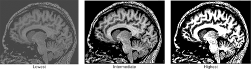FIGURE 2.4.1.2. Contrast. The effects of varying levels of contrast are shown for a single cross-sectional sagittal view of the brain. Contrast varies from lowest on the left and intermediate in the middle to highest on the right.

Brain Imaging Modalities

Computed Tomography (CT)

Computed tomography (CT or CAT scanning) uses x-ray beams to penetrate through body parts and provide views of internal body structures. The images in CT are generated by quantifying the degree of absorption of the x-ray beam by the
various body parts through which it passes. In a conventional x-ray, such as that of the chest or abdomen made for clinical diagnosis, all the organs through which the x-rays pass are collapsed onto the single, two-dimensional x-ray film, so that distinguishing the features of differing organs is difficult. CT imaging, however, uses an array of detectors placed around the subject to measure the reduction in strength, or attenuation, of multiple x-ray beams passing through the same body region from many different angles. Reconstruction of an image using attenuation measures from all of these beams gives an accurate representation of the tissues located at differing depths within the body through which the beam passes. CT has excellent depth penetration and sensitivity, although it provides low contrast to discriminate among various soft tissues. The spatial resolution of CT images is approximately 1 mm, and the imaging plane is limited to axial sections.

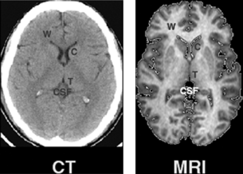FIGURE 2.4.1.3. MRI vs. CT contrast. The contrast obtainable by MRI and CT is compared in axial images acquired at the level of the basal ganglia. Contrast characteristics are vastly superior in MRI. Letters are shown overlaying various tissue types and anatomical structures: C = caudate nucleus (subcortical gray matter); T = thalamus; CSF = cerebral spinal fluid; W = white matter of the frontal lobes. (See color insert.)

In a so-called “spiral,” multidetector CT scanner, each detector records the transmitted x-ray beam as the source of the beam spirals around the body. Measurement of attenuation in beam intensity enters into a large set of equations used to calculate the densities of the tissues through which the beam has passed. These densities are mapped to each voxel of a set of thin 2D slices in the brain. When stacked one on top of another, many such 2D slices constitute a 3D imaging volume of the brain. Because the number of detectors and their packing density determines the resolution of the scanner, increasing the number of detector elements has become a major focus of the development of CT scanners. A higher number of detectors also enables a more rapid acquisition of individual slices. State-of-the-art CT scanners have tightly packed detectors that enable acquisition of up to 64 slices, thereby increasing brain coverage and the ability of CT to image smaller structures. Recently, hybrid PET/CT scanners have been constructed that combine the ability of PET to image blood flow and neurotransmitter systems with the ability of CT to provide high-resolution anatomical images of the brain. In addition, CT is being used to monitor the targeted delivery of medications and to individualize therapy for patients with cancer. Use of high-speed CT scanners in conjunction with administration of a contrast agent makes possible the measurement of blood flow in brain tissues, permitting the rapid assessment of possible stroke patients and evaluating the need for thrombolytic medications.

Positron Emission Tomography (PET)

PET uses radiotracers to track and then produce images of various In vivo biochemical and neurophysiological processes. Radiotracers are compounds of simple molecules, such as glucose, that are labeled with radioactive nuclei, such as ¹¹C and ¹⁸F, ¹³N, or ¹⁵O, that emit positrons after they are injected into the subject being imaged. Within a short distance (<3 mm) from the site where the positron is emitted, the positron collides with electrons that present naturally within molecules of the surrounding tissue. The colliding positrons and electrons annihilate one another, producing two gamma rays that are emitted at 180° trajectories from one another. These two gamma rays then pass out of the tissue and are recorded by detectors positioned in the axial plane surrounding the head. The precise localization of the origination of the gamma rays can be determined by noting which detections occur simultaneously at 180° orientations.

The locations where positrons (and the subsequent gamma rays) originate, and the information they provide about brain physiology, will vary depending upon the pharmacological properties of the particular radiotracer used. Some tracers, for instance, are located primarily to the intravascular space and are used to measure blood flow. Other tracers, like 2-deoxyglucose, are treated as energy substrates and thus are taken up by neurons and phosphorylated; because phosphorylated deoxyglucose cannot be metabolized, however, the radioactive tracer accumulates and can be measured as an index of the metabolic activity of the neurons containing them. Still other tracers act as ligands for specific neurotransmitter receptors, including various receptor subtypes for the dopamine, serotonin, and GABA receptors. The resolution of the images constructed using various tracers is determined in part by the tissue compartment in which the tracer is located, because this determines the distance between the site of positron emission and annihilation from each of the isotopes. In-plane resolution for typical PET scanners is 6 mm, while the newest high-resolution scanners have an improved in-plane resolution of 2 to 3 mm.

The radioactive isotopes used in the synthesis of various PET tracers have relatively short half-lives. The half life for ¹⁵O, which is incorporated into water molecules in studies of cerebral blood flow, is two minutes. That for ¹¹C, which is incorporated into various molecules that bind to neurotransmitter receptors, is 20 minutes; and that for ¹⁸F, which is incorporated into deoxyglucose for studies of brain metabolism, is 110 minutes. Because of these short half-lives, the radionuclides must be produced in a cyclotron located at or near the site of the PET scanner. The cost of constructing and maintaining this cyclotron contributes to the great expense of PET imaging relative to other imaging modalities.

Single Photon Emission Computed Tomography (SPECT)

SPECT is similar to PET in that it measures gamma ray emissions from minute amounts of radioactively labeled molecules that have been injected, ingested, or inhaled. Whereas PET tracers emit positrons that produce two gamma rays oriented at 180° trajectories from each other, SPECT tracers emit photons whose spatial orientations and times of emission, are independent of those for any other photon released— hence the “single photon emission” in the SPECT moniker. These photons pass through brain tissue and are subjected to scattering before they are detected and measured using collimators. The density and spatial organization of these collimators will determine the precision with which the
trajectories and sites of origin of the emitted photons can be determined. More collimators therefore improve the spatial resolution of a SPECT scanner. Increasing the number of collimators, however, also proportionately reduces the number of photons that enter each of the detectors and thus reduces sensitivity, or the SNR, of the scanner. Desires for improved resolution and SNR therefore must be weighed against one another with SPECT imaging, just as they are with other imaging modalities. The resolution of typical SPECT images is 6 to 10 mm, while newer scanners yield resolutions of 5 to 6 mm.

SPECT ligands typically incorporate isotopes of technetium and iodine, which have long half-lives and that therefore, unlike PET ligands, do not need to be synthesized on site in a large and expensive cyclotron. This is a major cost-saving advantage of SPECT compared with PET. In addition, the development of pharmacologically specific tracers is often easier with SPECT than with PET. Compared with PET, SPECT can detect slower kinetic processes because of the longer half-life of its tracers. The most common use of SPECT in the study of psychiatric diseases has been the measurement of regional cerebral blood flow, although it has also been used commonly to study neurotransmitter systems.

Magnetic Resonance Imaging (MRI)

In general use since the early 1980s, MRI is perhaps still most commonly regarded as a clinical tool that provides exquisite images of brain anatomy. MRI, however, has seen extraordinary growth in its use for studying brain activity associated with specific cognitive tasks, and more recently, it has also been used to study the concentration of certain metabolites and neurotransmitters in the brain, as well as to assess the integrity and orientation of nerve fiber tracts. To understand what these modalities can and cannot tell us about brain structure and function, one must become familiar with the basic processes by which MRI captures and represents within an image the features of brain structure and function.

Biological tissues are as much as 70 percent water by weight. Each water molecule contains two hydrogen atoms whose nuclei comprise a single proton each. MRI uses these single-proton nuclei to generate a radio signal from the brain that carries information about the microscopic environment in which the hydrogen nucleus finds itself. This information and the anatomical location from which it originated is decoded by computer software in the MRI scanner and then assigned an intensity (a level of grayness) within the corresponding pixel of the image. This intensity represents that quantity of the particular biological information encoded by the radio signal coming from the brain, which is selected and tuned by the scanner. The biological information being probed by the scanner determines the modality of the MRI study being conducted— i.e., whether it is studying the density of tissue in anatomical MRI, the oxygen content of the tissue in functional MRI, the diffusion of water in diffusion tensor imaging, or the concentration of certain neurometabolites in MRI spectroscopy. The brain is turned into a radiotransmitter through a combination of the powerful magnetic field within the MRI scanner and the transmission by the scanner of a series of pulses of radio waves that the brain tissue absorbs and then returns as another series of radio waves, now encoding the desired information about the tissue being imaged. We will now describe in greater detail precisely how this combination of magnetic field and radio waves from the MRI scanner turn the brain into a radio transmitter.

The nuclei of hydrogen atoms within biological tissues normally and inherently spin on an axis, like a spinning top or the earth. In the absence of a strong magnetic field, the axis of a spinning proton is oriented randomly in space. However, when biological tissues are placed within the powerful magnetic field of an MRI scanner, the spinning protons align in one of two directions, either parallel or antiparallel with the direction of the magnetic field (Figure 2.4.1.4). The number of protons aligned in parallel with the magnetic field is always slightly higher than the number of protons aligned antiparallel to the magnetic field. Because the magnetic fields produced by spinning protons aligned in opposite directions cancel each other, only the “excess” protons aligned parallel to the magnetic field contribute to the measurable radio signal used to generate an MR image. Nevertheless, because the numbers of molecules present in each cubic centimeter of tissue are enormous, the numbers of excess protons are still sufficient to produce a detectable and measurable signal. Thus, MRI has inherently low sensitivity in measuring the physical characteristics of brain tissue compared with other imaging modalities, because an MRI signal cannot be acquired from every molecule within a given voxel. On average, a few molecules per million participate in the process of image formation using MRI. At higher magnetic fields, the number of participating protons increases, hence providing the constant drive toward building scanners that operate at higher field strengths.

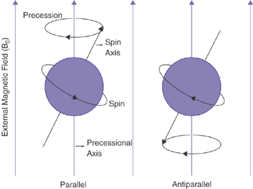FIGURE 2.2.1.4. Schematic representation of the alignment of spin magnetic dipole moment (m) with a strong external magnetic field (B₀). Only two spin states are allowed: one with m parallel to B₀ and one with m opposing or antiparallel to B₀.

In addition to spinning on an axis that is parallel to the magnetic field, these hydrogen nuclei also gyrate, or “precess,” when exposed to the magnetic field of the scanner, much like a spinning top or gyroscope in the presence of the earth’s gravitational field (Figure 2.4.1.4). Similar to the orientation of the spin of the proton, precession also occurs on an axis that is parallel to the magnetic field and at a particular frequency. The scanner then emits pulses of radiofrequency (RF) energy whose frequencies match precisely the frequency at which the protons are precessing. The coincidence of the two frequencies, that of proton precession and that of the RF pulses, creates the resonance effect of MRI through which the precessing protons absorb the energy within the RF pulses (the resonance frequency of precession happens to equal precisely the spin frequency of the protons). This absorption of energy excites the precessing protons, causing the axis of their spins to tilt toward the plane perpendicular to both the axis of precession and the static magnetic field. Following application of the RF pulse, the excited protons will slowly “relax,” tending to realign their spin axes with the main magnetic field. Because the spin itself of each proton creates a radio signal, the rate
of energy relaxation can be measured, a rate that differs from proton to proton depending on the nature of the surrounding tissue. Differences in the rate of relaxation between the protons of differing tissue types translate into contrast between those differing tissues types within an MR image. Application of additional magnetic field gradients in precise patterns too complicated to review here encodes the location of the proton emitting the signal. All MRI modalities use these same basic techniques to encode information about various physiological features and location of brain tissue.

MRI Modalities

Anatomical MRI

This imaging modality most often provides clinical information concerning the presence of localized lesions or anatomical defects within the brain. Most neuropsychiatric disorders, however, are not reliably associated with anatomical lesions that can be identified by gross inspection of the image. The utility of anatomical MRI in studying neuropsychiatric disorders therefore lies in its ability to provide more subtle information about brain structure— most commonly, information concerning the volumes and occasionally the shapes of particular brain regions. Although image resolution in most current anatomical imaging studies is approximately a cubic millimeter, in practice, the reliability of measures of regional brain volume is poor for structures smaller than a few cubic centimeters.

Image Analysis

The volumetric measurement of anatomical images depends critically on the methods used to analyze the images. Image analysis typically involves initial preprocessing steps, which tend to vary considerably from lab to lab. Preprocessing, however, usually involves some attempt to reduce the noise and improve the contrast of the images. One important step that is usually required, especially when a goal of analysis is the differentiation of tissue types across spatially distant portions of the brain, is correction of a systematic drift in intensity of the pixels that is caused by systematic and artifactual variation in the intensity within the image. Systematic and artifactual variation is produced by variations either in the magnetic field or in the radiofrequency pulse from the scanner that is used to turn the brain itself into a radio transmitter (3,4). This systematic drift in intensity will make some pixels that represent cortical gray matter, for instance, look more like higher intensity white-matter pixels.

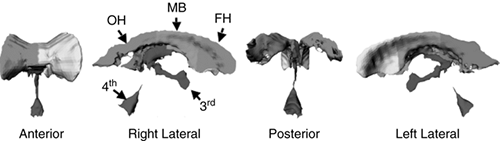FIGURE 2.4.1.5. Parcellation of the cerebral ventricles. After segmentation, the cerebral ventricles are parcellated. The lateral bodies of the ventricles are divided into three subregions using two coronal planes, one through the anterior commissure (AC) and one through the posterior commissure (PC). The temporal horns are separated from the lateral bodies using an axial plane containing both the AC and PC. The third ventricle is separated from the lateral ventricles at the foramen of Monroe, and the fourth ventricle is separated from the third at the top of the cerebral aqueduct. Subdivisions are shown in four views: anterior, right lateral, posterior, and left lateral. FH = frontal horn; MB = midbody; OH = occipital horn; TH = temporal horn; 3^rd = third ventricle; 4^th = fourth ventricle. (See color insert.)

The next steps in image analysis after preprocessing usually involve some way to differentiate one kind of tissue in the brain from another, termed tissue segmentation, and then subdivision of individual tissue types into subregions, a process termed tissue parcellation. Both of these steps may be performed using manual definition, computerized automation, or some combination of both. Segmentation may be used to help isolate brain from nonbrain tissues (i.e., in differentiating cortical gray matter from cerebrospinal fluid [CSF] in the sulci), in differentiating gray matter from white matter, or in differentiating CSF in the ventricles from surrounding white matter. Although the methods used to segment tissue types are many and varied (5,6,7,8,9,10,11,12), they all rely considerably on differences in pixel intensity across gray matter, white matter, and CSF. The simplest automated method of segmenting tissues is simply to define the tissue types based on a range of gray-level values, which typically is based on features of the histogram across the entire image or in some portion of it. Even the most sophisticated techniques for tissue segmentation rely to some extent on these image histograms.

Once tissues are segmented one from another, they often are subdivided to provide more anatomically relevant subregions. Cortical gray matter, for example, may be divided according to prefrontal, motor, sensory, or parietal cortices. Ventricular CSF may be divided into the lateral bodies, temporal horns, or the 3rd and 4th ventricles (Figure 2.4.1.5), subcortical gray matter might be divided into caudate, putamen, globus pallidus, and nucleus accumbens (Figure 2.4.1.6), and the cerebral hemispheres can be divided into a variable number of sections (Figure 2.4.1.7). Like segmentation, parcellation may be performed either manually or with the aid of computer automation. Parcellation may involve definition of borders and contours using primarily differences in the gray-scale intensity of the pixels across regions of interest. More automated methods of tissue parcellation include the use of natural boundaries between tissue types, such as the boundaries of cortical sulci and gray matter, to help subdivide gray matter of the cerebral cortex (13). The assumption, however, that divisions based on the cortical sulci follow boundaries between cytoarchitectonically unique subregions, such as those described in the classifications of Brodmann (14) or others (15,16) is true only to a first approximation (17,18). Another common method of tissue parcellation is the use of anatomical landmarks within the brain to divide tissues around those landmarks into subregions. These kinds of landmarks, such as the anterior and posterior commissures, are generally considered relatively invariant across individuals in their spatial relationship to other structures within the brain, although this assumption is largely untested (19,20,21).
A number of computerized methods using statistical models of shape have also been proposed for the more precise delineation of anatomical subregions in the brain; however, these methods require expert knowledge at various levels (22,23,24,25,26,27,28,29,30,31,32). These methods first learn shape (i.e., by computing various statistics of the shape) for a specific brain region from an example set of 20 or more regions that were previously delineated by an expert and then use these computed statistics to delineate the region in a new subject image. Most studies use some combination of these various parcellation schemes to define anatomical subregions within tissue types (33).

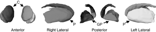FIGURE 2.4.1.6. Hand-tracing the basal ganglia. To delineate basal ganglia, the anatomical MR image was first cropped to the cortices surrounding the basal ganglia, and then the contrast between structures in the cropped image was enhanced by histogram equalization. Finally, we hand-traced the caudate, putamen, and globus pallidus nuclei in the transaxial plane. The head of the caudate nucleus was delineated from the accumbens nucleus by drawing a straight line in the coronal plane from the inferior tip of the internal capsule to the inferior tip of the lateral ventricles. C = caudate; P = putamen; GP = globus pallidus. (See color insert.)

A number of laboratories have introduced more novel, largely automated methods of image analysis that segment and parcellate much of the brain (34,35,36,37). These methods offer the promise of establishing large, normative databases in which the data from individuals and groups can be compared. Although the details of these methods of course vary considerably across laboratories, they tend to have in common with one another the warping of individual brains into a standardized brain space, so that a voxel in one brain is superimposed to the greatest extent possible on the corresponding voxel in another brain, called image coregistration. The simplest way to coregister images involves manual reformatting (rotation, translation, and scaling, and then reslicing) of one image (called the float) until the reformatted image superimposes on the other image (called the target) to the greatest extent possible. More advanced computerized methods use information (such as externally placed markers, pixel intensities, or other image features, including edges) from the images to be registered, and therefore are fast, consistent, precise, and do not require human interaction (38,39,40,41,42,43,44,45,46,47,48,49,50,51,52,53). Once images from differing subjects are coregistered, the methods then either find some way to measure the deviation of each voxel in one individual or group from the mean of the sample or from the mean of another group. Any number of characteristics can be compared across groups, but common features include estimates of relative volume, shape, thickness of the cortical mantel, or correlations of these local brain-based measures with the clinical measures of subjects at particular points of the cerebral surface (Figure 2.4.1.8), local white matter intensities, and volumes of the subcortical nuclei.

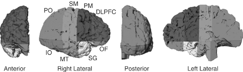FIGURE 2.4.1.7. Parcellating right hemisphere into eight anatomical sectors. Here the brain is isolated by using an isointensity contour function in conjunction with manual editing. We then used a curvilinear plane positioned through standard midline landmarks to divide the brain into hemispheres. We used one axial plane containing the anterior-commissure (AC) and posterior-commissure (PC), and three coronal planes (one tangential to the anterior border of the AC, one through the PC, and one tangential to the genu of the corpus callosum) to divide the right hemisphere into eight anatomical sectors. DLPF = dorsal prefrontal; PM = premotor; SM = sensorimotor; PO = parietooccipital; IO = inferior occipital; MT = midtemporal; SG = subgenual; OF = orbitofrontal. (See color insert.)

Applications

Anatomical MR images have been extensively used to define brain structures and to study correlates of brain measures, including volumes of entire structures and local changes in volumes, with various clinical and genetic measures within and across groups of subjects (54,55). Additionally, because anatomical MR images have high spatial resolution, SNR, and tissue contrast, these images are used for anatomical localization of brain activations and deactivations in functional MR studies, white matter fiber pathways in diffusion tensor studies, and concentration of brain metabolites in MR spectroscopy studies. Furthermore, anatomical MR images play the key role in coregistering unique information from various MR modalities within a multimodal framework that will greatly help an investigator to constrain interpretations regarding the neural bases of developmental psychopathologies.

Limitations

Measurements of regional brain volumes tell us little or nothing about the brain’s ultrastructural features, such as the number, anatomical integrity, or connectivity of the cellular elements that constitute the volume of the tissue being measured. The
ultimate significance of individual or group differences in regional volumes that can be detected by imaging studies is therefore still an open question. Nevertheless, recent clinical and preclinical studies suggest that individual variance in the macroscopic volumes that we measure on MR images may arise from genetic differences (56) as well as from experience-dependent effects (57) that influence the addition, subtraction, or reorganization of cellular elements within that volume. These effects of neural plasticity are known to influence brain structure at all levels, from the remodeling of synaptic architecture to the organization of cortical maps (57,58,59). Volumetric data may therefore carry information about the effects of genetic liabilities and past experiences on the macroscopic structure of the brain.

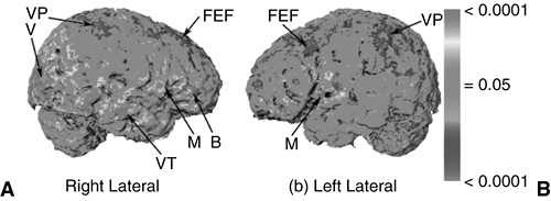FIGURE 2.4.1.8. Correlating IQ and shape. Statistical analyses of the correlations between intelligence quotient (IQ) and the shape of the cortex for a group of 32 healthy subjects. The color-encoded p-values of the correlations (violet denotes negative and red denotes positive) between IQ and cortical surface are plotted across the entire surface of the cortex of a subject selected as reference. B = Broca’s region; FEF = frontal eye fields; M = motor; V = vision; VP = visual parietal; VT = visual temporal. (See color insert.)

Functional MRI

The discovery that the MRI signal represented in the gray-scale values of an MR image can, when tuned to encode certain features of the volume being imaged, vary during performance of a cognitive or behavioral task was first reported in 1991 (60). This time-varying signal has been found to reflect primarily changes in deoxyhemoglobin concentration within the corresponding voxel of the brain. Deoxyhemoglobin concentration is a complex function of the temporal variation in oxygen use and blood supply (termed the blood oxygen level dependent or BOLD response), which ultimately depends on the corresponding temporal variation in the activity of neurons within that voxel. The change in MRI signal during a task is therefore an indirect measure of the change in neuronal activity associated with the performance of that task.

FMRI Time Series

The variation in fMRI signal associated with performance of a task is monitored and tested statistically by acquiring many images in rapid succession while subjects perform in alteration at least two tasks, one of which is the baseline (or control) task and the other of which is the primary task of interest. A typical fMRI experiment might acquire an image in each slice every 1–2 seconds, for a total of several hundred to several thousand images per experiment in that slice per subject. The signal within any single pixel at the times of acquisition of those images will therefore constitute a time-ordered series of signal values, or an fMRI time series. If the neuronal activity within a voxel of brain tissue varies systematically through time with the change in performance of one task to the other, the signal in the corresponding pixel’s time series will also vary systematically through time with the change in task (Figure 2.4.1.9). The time-dependent variation in the fMRI signal or, equivalently, in the pixel’s gray scale, can then be tested statistically to determine whether it varies with the change in task at a level that is beyond chance. Although this task-dependence of the time-varying fMRI signal can be tested using many more or less sophisticated statistical procedures, the simplest is to sort the signal values of the time series into two populations— those acquired during the baseline task and those acquired during performance of the primary task of interest. The means of these populations of signal values are then tested using any number of parametric or nonparametric statistics, the most common of which is a t-statistic (Figure 2.4.1.10). The magnitude of the t-statistic or its corresponding probability value is typically color-coded and then painted on the pixel of the image that represents a voxel in the corresponding slice of brain. Pixels in which the t– or p-value surpasses a predefined threshold are then considered “active” during the primary task of interest relative to the baseline task. FMRI methodologies depend critically upon comparing signal intensities within each pixel across two or more tasks to determine where in the brain neural activity varies systematically with the change in performance of one task to another.

Only gold members can continue reading. Log In or Register to continue