Fig. 12.1
Pipeline of the K-complex detection methodology
First step: In the first step, all the local minima from each available signal are detected and considered as candidate K-complexes. The peaks should have at least a minimum absolute peak height and be at least separated by a distance threshold; thus smaller peaks that may occur in close proximity to a large local peak are ignored. The center of each candidate K-complex is defined as the location of the local minimum. The idea is to limit the number of the candidates using a multi level approach. At each level a new feature related to a rule is calculated. If the value of the feature complies with the rule, the candidate passes on to the next level, otherwise the candidate is rejected.
The first feature is the peak to peak amplitude. The algorithm checks if the local minimum is followed by a positive component and computes the value of their peak to peak amplitude. Then a 10 second epoch around the local minimum is extracted from the EEG signal and a segment of 1 second epoch prior and following the minimum are removed, yielding an epoch indicating the background. The standard deviation of the background EEG amplitude is calculated and the following rules are checked:
Rule 1: The peak to peak amplitude should be greater than three times the amplitude of the background EEG and between 70 and 560 μV. Also the standard deviation of the wave should be 1.2 times larger than the standard deviation of the background.
Rule 2: The duration of the negative sharp wave should not be lower than 300 ms and greater than 1 s.
Rule 3: All the frequencies more than 20 Hz should not have power greater than the 3 % of the total power of the signal. Otherwise it is assumed that muscle noise is contaminating the data.
The candidates remained from the application of the rules in each channel are fused with the data integration procedure summarized in rule 4: rule 4: The candidate wave should be detected at least in three channels to be a K-complex.
The majority of false detections even after the application of the above rules in our experiments are delta waves. Delta waves are similar to K-complexes and occur mainly in Slow Wave Sleep. Their characteristic is the fact that they occur repeatedly compared to the single appearances of K-complexes. In order to exclude delta waves from the set of candidates, we apply a simplified estimation of the Slow Wave Sleep epochs and we reject candidates belonging to them. Such a simplified estimation of Slow Wave Sleep is achieved by computing the frequency of appearance of the detected candidates in 10 s epochs. If the frequency of the detected candidates reaches a threshold, all the candidates belonging to the epoch are rejected because it is assumed that the epoch belongs to sleep stage 3 or 4. The threshold is an appropriate percentile of frequency of K-complex appearance estimated by whole night sleep recordings.
Rule 5: Candidates in very close proximity to each other are rejected.
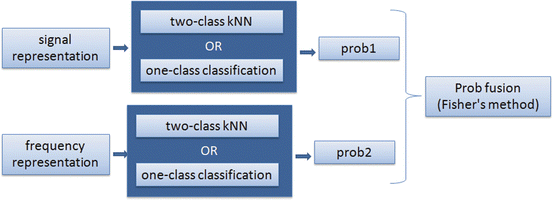
Second step: The remaining candidates after applying the aforementioned rules are given as input to a classifier. In this step, we implemented two different classification methods; a k-nearest neighbor (kNN) classifier, which uses training samples from both classes (K-complexes and false detections) and a one-class classifier, which uses training samples only from the positive class (K-complexes). Both classifiers use as input two different representations of the waveforms, the signal and frequency representation and produce a decision function indicating the probability of the input sample to be a K-complex. The two pseudo-probabilities (by each representation) are then fused by Fisher’s method and thresholded to obtain the final decision. A schematic diagram of this step is shownabove (Fig. 12.2).


Fig. 12.2
Schematic diagram of K-complex classification (second step of the automatic detection methodology)
KNN classifier uses a training set containing false detections from the first step and true K-complexes, which is balance the by applying k-means clustering in the class with more training samples. For each test sample, the kNN classifier computes the distance to each training sample. The distance is calculated either as Euclidean distance (if fast performance is targeted) or by applying Optimal Subsequence Bijection (OSB) (if accuracy is targeted). OSB is a distance function proposed in [1] and is appropriate for time series. OSB first computes an elastic matching of the two sequences and then calculates the distance using the distances of corresponding elements. Since both the query and the target sequences may be noisy, i.e., contain some outlier elements, the idea is to exclude the outlier elements from matching in order to obtain a robust matching performance.
The test sample’s probability of being a K-complex is calculated as the ratio of the number of nearest neighbors being K-complexes divided by the total number of nearest neighbors, k. The two pseudo-probability vectors (for the signal and frequency representation) are fused by Fisher’s method [2] which combines p-values from several independent tests into one test statistic that has a chi-squared distribution. Based on the fused vector of probabilities, a test sample is assigned to the K-complex class if its probability is above a threshold. Otherwise, the test sample is considered as non K-complex.
The one-class classifier uses a training set containing only K-complexes as training samples. The spectral clustering algorithm proposed by [3] is applied to the training set, producing a set of clusters. The resulting clusters represent the different patterns of the K-complex. The distribution of the samples within each cluster is learned by calculating all pairwise distances. Given the training clusters, the one-class classifier assigns to a test sample a probability of being an outlier (non K-complex) if it deviates from the learned distribution as following. The test sample’s distance to each cluster is calculated as the distance to the closest sample in each cluster. The test sample is then assigned to the closest cluster and the significance level (p-value) of the calculated distance for the specific cluster is returned as pseudo-probability of being an outlier.
The method was evaluated on an all night sleep EEG recording collected from a healthy female subject with sampling frequency 2500 Hz. The recording contains 14 excerpts each 30 min long. Before running the detector, each excerpt had been annotated manually by an expert neurophysiologist. In the whole recording 278 K-complexes were manually annotated. The detections of the algorithm were compared to those of the expert. The performance of the detection algorithm was evaluated by calculating the true positive rate (TPR) and the false positive rate (FPR). The True Positive Rate of the kNN classifier used with the OSB distance function was 77 % while False Positive Rate was 29 %. The corresponding confusion matrix, which reports the numbers of K-complexes detected by the algorithm and the expert, is illustrated in Table 12.1 (on the left).
Table 12.1
Confusion matrix for kNN and one-class classifier (UoP dataset)
Expert | |||||
|---|---|---|---|---|---|
kNN classifier | One-class classifier | ||||
Algorithm | K-complex | Non K-complex | K-Complex | Non K-complex | |
K-complex | 214 | 949 | 211 | 1324 | |
Non K-complex | 64 | – | 67 | – | |
Similar results were obtained by the one class classifier. A True Positive Rate of 76 % was obtained with about 43 % False Positive Rate. Table 12.1 (on the right) illustrates the respective confusion matrix.
Our method was also evaluated in a dataset, which consists of ten excerpts of 30 min EEG recordings, coming from more than one healthy subjects. The dataset is available for use by the University of MONS—TCTS Laboratory and Universite Libre de Bruxelles—CHU de Charleroi Sleep Laboratory. The sampling frequency was 200 Hz. This time, the kNN classifier obtained a 73 % TP rate for 33 % FP rate. The respective statistics for the-one class classifier are 76 % TP rate and 41 % FP rate.
12.2.2 Detection of Sleep Spindles
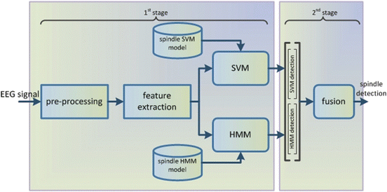
For the detection of sleep spindles we relied on the combination of discriminative and statistical models. Specifically, the support vector machines and the hidden Markov models (HMMs) were selected due to their advantageous performance in similar signal processing tasks. The sleep spindle detection is performed in two stages. In the first stage the signal is pre-processed, parameterized and processed independently from the discriminative (SVMs) and the statistical (HMMs) models. In the second stage the output recognition results from each model are combined by a fusion method in order to provide the final sleep spindle detection results. The block diagram of the proposed scheme is illustrated in Fig. 12.3.


Fig. 12.3
Block diagram of the combined SVM-HMM sleep spindle detection scheme
As shown in Fig. 12.3 an EEG signal is introduced to the system and pre-processed with framing of the signal to blocks of L samples. Each frame is time-shifted by its preceding one by s samples, where  , thus resulting to overlapping frames. At the feature extraction block for each of the computed frames a parametric vector is computed by a signal parameterization algorithm.
 , thus resulting to overlapping frames. At the feature extraction block for each of the computed frames a parametric vector is computed by a signal parameterization algorithm.
The output of the feature extraction block is forwarded in parallel to each of the two models, i.e. the discriminative SVM-based and the statistical HMM-based sleep spindle models. Each of the two models estimates whether each incoming feature vector corresponds to sleep spindle or not, i.e. providing binary classification results with the corresponding recognition score for each of the two classes.
The second stage of the sleep spindle detection scheme exploits the recognition results of the two models, i.e. the SVM-based and the HMM-based, in order to combine them and provide a final decision for each feature vector. Specifically, the recognition results estimated at the first stage by each of the two models, are concatenated in a single vector as shown in Fig. 12.3. A fusion model utilizes the SVM-based and HMM-based predictions, which are included in the single vector, in order to provide the final decision for each frame of the EEG signal. In the present work the fusion model was implemented with the SVM algorithm. For the implementation of the SVM and the HMM models we relied on the WEKA and HTK software toolkits.
The performance of the proposed combined SVM-HMM sleep spindle detection scheme was evaluated on EEG data recorded at the Medical School of the University of Patras. The EΕG data were recorded at sampling frequency of 2500 Hz, using 64 channels. For the present evaluation we used the CZ electrode recordings from one subject. The duration of the evaluated data is approximately 401 minutes. The sleep recordings were manually annotated by expert sleep technicians of the University of Patras. The evaluated data include 1228 occurrences of sleep spindles and no overlap between training and test data subsets existed. The sleep spindle detection performance is shown in Table 12.2.
Table 12.2
SVM-HMM sleep spindle performance (in percentages)
Recognized as → | Spindle | Non-spindle |
|---|---|---|
Spindle | 88.54 | 11.85
Stay updated, free articles. Join our Telegram channel
Full access? Get Clinical Tree
 Get Clinical Tree app for offline access

|


