Quantitative Genetics
Anita Thapar
Peter McGuffin
Patterns of inheritance
Our understanding of how traits and disorders are passed from one generation to the next began with the work carried out by an Augustinian monk, Gregor Mendel. Although Mendel’s published work in 1866 was initially ignored, its rediscovery at the beginning of the twentieth century heralded the beginning of modern genetics. Mendel’s experiments on pea plants and his observations of the patterns of inheritance of certain characteristics led to the development of his particulate theory of inheritance. It was only later in 1909 that the units of inheritance that he had described were named genes and alternative forms of a gene were termed alleles. It was also at this time that the terms phenotype, used to describe the observed characteristic, and genotype, used to refer to the genetic endowment, were introduced.
Mendel’s laws
Mendel examined clear-cut dichotomous characteristics such as smooth versus wrinkled coats in peas. He first noted that when parents of different types were crossed, the first generation (F1) offspring displayed uniformity of that characteristic. He inferred that this uniformity was due to one phenotype being dominant and the other being recessive. Thus, when homozygous parents AA and aa produced heterozygote Aa offspring, these offspring displayed the phenotype of the AA parent rather than manifesting a phenotype intermediate to those of both parents.
Mendel then demonstrated that when the F1 heterozygotes (Aa) were intercrossed (Aa × Aa), segregation resulted in the second F2 generation showing recessive and dominant phenotypes in the ratio of 1 to 3. He then inferred that this F2 generation consisted of three types (AA, Aa, and aA, aa) occurring with a probability of 1:2:1.
Finally, Mendel showed that when the transmission of two different phenotypic traits was studied, they showed independent assortment. We now know that independent assortment occurs when the genes coding for these traits are either located far apart on the same chromosome or are on different chromosomes (see linkage).
Single-gene disorders
Although disorders showing a simple Mendelian pattern of inheritance are rare, they tend to be clinically severe and collectively impose a significant burden.
For autosomal dominant disorders to manifest themselves, only one disease allele is necessary, i.e. both heterozygotes as well as homozygotes (those who carry both disease genes) will be affected. In most instances, where there is one affected parent who is a heterozygote for the disease, approximately 50 per cent of the offspring will show the disorder. Autosomal disorders tend to be severe and manifest themselves in every generation. Huntington’s disease and acute intermittent porphyria are examples of autosomal dominant conditions that are often present with psychiatric symptoms.
Autosomal recessive conditions such as phenylketonuria require the presence of two disease alleles to show clinical manifestations of the disorder. Thus, they often appear to skip generations. These disorders usually occur in the offspring of two ‘carrier’ heterozygote parents and are more common where there is a high rate of consanguinity (e.g. marriages between cousins) as these inbred populations will show greater homozygosity at all loci.
The other group of single-gene disorders consists of sex-linked conditions such as fragile X syndrome. Normal females have two X chromosomes whereas normal males have one X chromosome and one Y chromosome. Thus, for recessive disorders on the X chromosome, if the mother is a carrier (X*X) and assuming that the father is unaffected (XY), half of her sons will manifest the disorder (X*Y) and half of her daughters will be carriers (X*X). Where the father is affected by an X-linked recessive condition, all the daughters will be carriers. As sons have to inherit their
X chromosome from their mother, there will be an absence of father to son transmission. X-linked dominant conditions are extremely rare.
X chromosome from their mother, there will be an absence of father to son transmission. X-linked dominant conditions are extremely rare.
Continuous traits
Mendel’s laws are based on the transmission of dichotomous characteristics, yet many important human phenotypes such as height, weight, and blood pressure are continuously distributed. However, we are able to show that Mendelian principles can also be applied for these types of quantitative traits.
Let us first consider a phenotype measured on a continuous scale which results from the influence of a single gene with two alleles A1 and A2 (see Fig. 2.4.1.1). We can now describe the phenotypes of the three possible genotypes in terms of a quantitative value on the continuous scale. A1A1 has a value of –a; A2A2 has a value of +a; and A1A2, the heterozygote, has a value of d. When d = 0, A1A2 lies exactly half way between A1A1 and A2A2, that is the genetic contribution is entirely additive. When d = –a, A2 is recessive to A1and when d = +a, A2 is dominant to A1.
At the simplest level, we assume that there are no dominance effects and that there is no mutation, selection, migration, or inbreeding in the population. If p is the frequency of allele A1and q is the frequency of A2 in the population where p + q = 1 then the frequency of genotypes can be expressed as follows:
A1A1A1A2A2A2
p2 2pq q2
This is known as the Hardy-Weinberg equilibrium. If we now simplify further and state allelic frequencies where p = q = 0.5, then the phenotypic values of A1A1, A1A2, and A2A2 would be distributed in the population with relative frequencies of 1:2:1.
Now if we consider a trait which results from two genes each of which has two alleles of equal frequency and additive effect, there would be five possible phenotypic values with relative frequencies of 1:4:6:4:1. Overall as the number of genetic loci (n) increases, the number of phenotypic values increases (2n + 1) and the distribution of phenotypic values more closely approximates a normal distribution. It is thought that most quantitative or continuous traits result from the additive action of genes at many loci which is otherwise known as polygenic inheritance. Where familial transmission is explained by environmental factors as well as by multiple genes, we then call this a multifactorial mode of inheritance.
Complex disorders and irregular phenotypes
(a) Polygenic/multifactorial threshold models
Most common human psychiatric and medical disorders such as schizophrenia, diabetes, and heart disease do not show a Mendelian pattern of inheritance. Neither can they be considered as continuous traits in that people are described as being affected or unaffected. However, these conditions could be regarded as quasi-continuous in that those who are affected can be graded along a continuum of severity. It is possible to extend this to assume that there is an underlying liability to develop the disorder which is continuously distributed in the population. Those who pass a certain threshold manifest the condition. If the underlying liability to develop the disorder is inherited in a polygenic or multifactorial fashion, then we can assume that the distribution will be approximately normally distributed (Fig. 2.4.1.2). The genetic liability of relatives of affected individuals will be increased and their liability distribution will be shifted to the right (Fig. 2.4.1.2). Thus, the proportion of relatives above the disease threshold will be greater compared with the general population. If we know the proportion of affected relatives of probands and the proportion of those affected in the general population, it is possible to calculate the correlation in liability between pairs of relatives using this type of model.
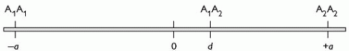 Fig. 2.4.1.1 A phenotype, measured on a continuous scale, resulting from a single gene with two alleles A1 and A2. |
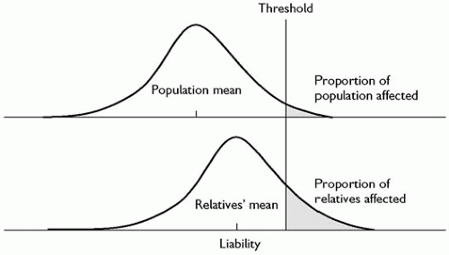 Fig. 2.4.1.2 A polygenic or multifactorial threshold model of disease transmission. |
(b) Single major locus model and atypical patterns of Mendelian inheritance
An alternative to a polygenic model of complex disease is a single major locus model. Single-gene disorders do not always show typical Mendelian patterns of inheritance. For example familial transmission can be modified by variable expression and penetrance. Some conditions can show great variability in terms of clinical expression. For example neurofibromatosis, an autosomal dominant disorder can express itself as the full blown disorder or merely as a few café-au-lait spots. Penetrance is defined as the probability of manifesting the disorder given a particular genotype. For Mendelian disorders this is always 1 or 0, but irregular patterns of inheritance may occur because of incomplete penetrance where the probability of manifesting the disorder is greater than 0 but less than 1.
Finally, there are now molecular explanations for other types of unusual patterns of inheritance for single genes. Anticipation where disorders show a progressively earlier onset and greater severity with subsequent generations is now known to be explained by heritable unstable nucleotide repeat sequences (see later). Huntington’s chorea and fragile X syndrome are examples of disorders caused by heritable unstable repeats. For some conditions such as the Angelman syndrome and the Prader-Willi syndrome, manifestation of the disorder depends on the parental origin of the gene. This is known as imprinting.
(c) Other models
Alternative explanations of how complex conditions such as psychiatric disorders are inherited include mixed and oligogenic patterns of transmission. A mixed model includes a major gene and a polygenic/multifactorial contribution. However, for many of these disorders, genes of major effect may not exist. It may be that these irregular phenotypes are best explained by oligogenic models where the co-action or interaction of a small number of genes contributes to the disorder. These issues remain to be resolved by molecular genetic studies (see later).
Components of phenotypic variation
We will now consider the different influences that contribute to phenotypic variation in a population. The total variation in an observed trait (phenotype vp) at the simplest level (ignoring non-additive effects) can be partitioned into a proportion due to genetic influences (vg), a component explained by shared environmental factors (vc), and a remainder accounted by non-shared environmental factors which includes error (ve):
vp = vg + vc + ve
Shared or common environmental influences are aspects of the environment that result in greater similarity of family members for a given phenotype. Non-shared environmental factors refer to environmental influences that have effects which are specific to individuals and that contribute to phenotypic differences between family members.
Although we have so far only considered one type of genetic contribution, the genetic variance vg can be further subdivided into variance due to additive genetic influences (va) and dominance effects (vd).
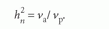
The relative influence of genetic factors is expressed as heritability and when defined as the proportion of the total phenotypic variance attributable to additive genetic variance, is known as narrow-sense heritability:
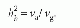
Heritability is also sometimes used to describe the proportion of variance explained by the total genetic variance (additive and non-additive genetic variance) and it is then known as broad-sense heritability:
Similarly we can estimate the proportion of the total phenotypic variance explained by shared environment where c2 = vc/vp and the remaining proportion attributable to non-shared environmental factors and error (e2).
It is important to remember that the estimate of heritability and the contribution of shared environment and non-shared environment are proportions of total variation within a given population, i.e. these parameters tell us about sources of difference between individuals in a population and have no meaning at an individual level. For example, if an individual was selected from a population where IQ had been shown to have a heritability of 50 per cent, it could not be said that 50 per cent of that individual’s IQ was determined by genes. Another important point is that these estimates are specific to the population studied and may differ for other populations. Finally, the contribution of genetic and environmental influences to a phenotype does not allow any inferences about the extent to which that phenotype is modifiable by environmental factors. For example, phenylketonuria is a Mendelian condition that is determined by the presence of a single-gene mutation. Yet the clinical manifestations of the syndrome are prevented by dietary intervention.
Non-additive genetic effects
So far we have simplistically assumed that phenotypic variation is influenced in an additive fashion. However, the contribution of genes and environment is more complex than this. We have already referred to genetic dominance effects where there is non-additive interaction of alleles within a locus. Another potential source of influence is the non-additive interaction between alleles at different loci which is known as gene-gene interaction or epistasis.
Gene-environment interaction
Gene-environment interplay represents another important form of non-additive genetic contribution to complex phenotypes.(1) The term gene-environment interaction (G × E) is used here to refer to individual genetic differences in response to specific environmental factors. In the presence of gene-environment interaction, individuals who are at genetic risk of a disorder do not manifest the condition unless they are exposed to a specific environmental risk factor. Gene-environment interaction also means that not all those exposed to an environmental risk factor will show disorder. Later, we consider direct investigation of gene-environment interaction through molecular genetic studies. Twin and adoption study designs have also been used to examine G × E, in an indirect way. Here, genetic liability is inferred by virtue of having affected relatives rather than through possession of a specific genetic risk variant.
Gene-environment correlation
Gene-environment correlation further adds to the complexity of interplay between genes and environment. Gene-environment correlation arises when a person’s genotype is correlated with the environment that they are exposed to. For example, sociable parents not only endow their children with genes but also provide an environment that encourages greater sociability in their children (passive gene-environment correlation). Moreover, positive gene-environment correlation would result where a sociable child actively seeks out more situations where socializing occurs (active gene-environment correlation) or where he or she evokes friendly responses in others (evocative gene-environment correlation). There is evidence that many important environmental risk factors in psychiatry (for example, life events) do correlate with genetic risk for specific disorders (for example, depression). Where that is the case, genetically sensitive designs are needed to investigate whether environmental risk factors have true environmentally mediated risk effects on disorder or whether the association has arisen because of genetic factors contributing to both the environmental risk exposure and disorder.
The presence of gene-environment interaction and gene-environment correlation highlights that the action of genes and environment must be considered together. Another important point is that in traditional twin study designs, G × E and G – E correlation effects are subsumed within the heritability estimate or in some circumstances the environmental variance component (see twin studies).
Research methods
Family, twin, and adoption studies
So far we have considered the theoretical basis of inheritance and possible sources of phenotypic variation and familial resemblance. Clearly, the investigation of the genetic basis of psychiatric disorders first requires us to examine to what extent genes and environment contribute to a given disorder or trait. Secondly, we need to know how genes and environmental influences exert their risk effects and finally we have to investigate the genetic basis of disorders at a molecular level.
Traditional methods in psychiatric genetics research include family, twin, and adoption studies. Family studies enable us to examine to what extent a disorder or trait aggregates in families. Familiality of a disorder can of course by explained by shared environmental influences as well as by shared genes. Twin and adoption studies allow us to disentangle the effects of genes and shared environment.
Family studies
(a) Methods
Family studies allow us to determine whether a disorder aggregates in families by examining the rate of disorder in the relatives of affected individuals (probands) and comparing this with the rate of disorder in the general population or in a control group. Alternatively we can compare the frequency of disorder in the relatives of probands with the frequency among relatives of a control group of normal individuals or those with another disorder.
There are two types of family studies. The family history method is more economical in that the psychiatric history is taken from the proband. However, given that most individuals are unlikely to know as much about family members as about themselves, this method results in an underestimate of diagnoses in relatives. A more thorough but more time-consuming approach is the family study method where all available relatives are directly interviewed.
(b) Ascertainment
An important issue is how a family study sample is ascertained. Ideally, probands should be ascertained independently from each other. This is unlikely to pose a problem for rare disorders. However, for more common conditions where a series of cases is collected, for example, by consecutive referrals of the disorder to a particular hospital, it is possible that families included in a family study contain more than one proband. This is known as multiple incomplete ascertainment. Complete ascertainment, where all affected individuals in a given population are included, is rarely possible and in most instances probands are identified after some selection process (e.g. referrals to a particular hospital). Thus, factors influencing selection, such as comorbidity and help seeking may also influence observed patterns of familial aggregation.
(c) Age correction
For genetic studies, we are interested in the proportion of individuals who have ever had the disorder (lifetime prevalence) rather than the proportion who show the disorder at one point in time (point prevalence). However, a difficulty encountered when carrying out family studies is that the observed rates of disorder will also depend on the age of the individual, the risk period for the disorder, and whether or not the individual has lived through that risk period. Thus, some members may not yet have reached the age of risk for the disorder, some are currently unaffected but will become affected at some later point, and others may have died whilst still unaffected. The most appropriate method is to correct for age and express the rate of disorder in relatives as the morbid risk (MR) or lifetime expectancy.
There are many methods of age correction, of which the Slater-Stromgen adaption of Weinberg’s shorter method is the most straightforward. The MR of the disorder can be estimated as the number of affecteds (A) divided by the bezugsziffer (BZ) where the BZ is calculated as:
Σi[a1]wi + A
and where wi is the weight given to the ith unaffected individual based on their current age. The most accurate approach is to use an empirical age of onset distribution from a large separate sample, for example a national registry of psychiatric disorders, to obtain the cumulative frequency of disorder over a range of age bands, from which weights can be derived.
Another approach is to carry out life table analysis. The distribution of survival times (or times to becoming ill) is divided into a number of intervals. For each of these one can calculate the number and proportion of subjects who entered the interval unaffected and the number and proportion of cases that became affected during that interval as well as the number of cases that were lost to follow-up (because they had died or had otherwise ‘disappeared from view’). Based on these, the numbers and proportions ‘failing’ or becoming ill over a certain time interval (usually taken as the entire period of risk) can be calculated. A further alternative is to use a Kaplan Meier product limit estimator. This allows one to estimate the survival function directly from continuous survival or failure times instead of classifying observed survival times into a life table. Effectively this means creating a life table in which each time interval contains exactly one case. It therefore has an advantage over a life table method in that the results do not depend on grouping of the data.
Twin studies
Identical or monozygotic twins, by virtue of arising from the fertilization of one egg, share 100 per cent of their genes. Non-identical or dizygotic twins are from two fertilized eggs and like full biological siblings share on average 50 per cent of their genes. Thus, assuming that monozygotic twins and dizygotic twins share environment to the same extent, monozygotic twins would share greater similarity than dizygotic twins for a disorder that is genetically influenced. Twin studies are an important method for disentangling the effects of genes and shared environment and can be used to estimate the contribution of genetic influences, shared environmental factors and non-shared environmental factors to the total variation for a given trait or disorder.
For continuous traits, twin similarity is expressed as an intraclass correlation coefficient where:
rmz = h2 + c2
rdz = 0.5h2 + c2
Thus, from observed monozygotic and dizygotic correlations for a given trait we can calculate heritability from the above equations where h2 = 2(rmz – rdz), c2 = 2rdz – rmz, and e2 is the remaining variance = 1 – h2 – c2 (see path analysis below).
For dichotomous characteristics (e.g. affected with a disorder and unaffected), twin similarity is expressed as concordance rates. A pairwise concordance rate is estimated as the number of twin pairs who both have the disorder divided by the total number of pairs. However, where there has been systematic ascertainment, for example a twin register, it is preferable to report a probandwise concordance rate which is calculated as the number of affected twins divided by the total number of cotwins.
(a) Ascertainment
One potential source of bias in twin studies stems from ascertainment procedures. For example, affected twins referred to a specific study or volunteer samples are likely to include more twin pairs who are monozygotic and who are concordant. Ascertainment of twin pairs through hospital registers overcomes this problem to some extent, but for some disorders may be biased by the process of referral. Population-based samples overcome these biases, although when examining disorders rather than traits extremely large sample sizes are required to obtain an adequate number of affected individuals.
(b) Zygosity
A further potential source of error is in the assignment of zygosity. Ideally zygosity should be determined by DNA typing. However, it may be more practical to use a twin similarity questionnaire which includes questions such as whether the twins share the same hair/eye colour, and whether they look alike as two peas in a pod. This method of assigning zygosity is simple and inexpensive with a reported accuracy of over 90 per cent.
(c) Equal environments assumption
It is sometimes argued that a major drawback to the twin study method is that monozygotic twins may experience a more similar environment and may be treated more similarly than dizygotic twins. However, where there is evidence that monozygotic twins share greater environmental similarity than dizygotic twins it is difficult to infer whether this contributes to their similarity for the disorder or whether this is the consequence of greater genetic similarity. There have been several approaches adopted to further explore this issue.
In some studies questionnaire measures of environmental sharing (e.g. being dressed alike as children, sharing friends) have been used. These suggest that environmental sharing is indeed greater for monozygotic twins than for dizygotic twins. However, it appears that for many traits and disorders such as cognitive ability, personality, depressive symptoms, and depressive disorder this degree of similarity for childhood environment does not account for monozygotic twin similarity for the trait. One way of disentangling cause and effect is to use direct observational studies. Although this method has not been much used, one study of young twins suggested that the greater similarity of parental responses to monozygotic twins compared to dizygotic twins appeared to be elicited by the twins themselves.
An alternative method of examining the effects of environmental sharing is to study twins who are mistaken about their zygosity. However, most studies which have used this method suggest that perceived zygosity is a less important influence on twin similarity than true zygosity.
Finally, the most powerful means of examining the effects of environmental sharing is to look at monozygotic twins who have been reared apart. However, such twin pairs are rare and have mostly been ascertained in a biased fashion. Nevertheless, studies of reared-apart twins have informed us that there is a substantial genetic contribution to cognition, personality, and psychosis.
(d) Comparability of twins
The final potential criticism of the twin method is whether twins can be regarded as representative of the general population given some important differences. Twin births are relatively common (1 in 80 births), although the number of dizygotic twins varies in different countries and is influenced by factors such as maternal age and multiparity, a family history of twins and increasingly, the use of fertility drugs. Twins are more likely to experience greater intrauterine and perinatal adversity and the experience of being brought up as a twin is unusual in itself. There is also some evidence that depression is more common in mothers of young twins than among mothers of singletons. However, these differences are only important if they result in different rates of disorder or symptoms in twins compared to singletons. So far there is little evidence to suggest that the rate of psychiatric disorder in twins is any higher than amongst singletons.
Related posts:


Stay updated, free articles. Join our Telegram channel

Full access? Get Clinical Tree


