Fig. 1
VR scenario used for visual stimulation. This snapshot shows one flash event of an object
2.3 Paradigm
The oddball paradigm we employed is designed to elicit a P300 potential which is a deflection of sensor values evoked approximately 300 ms after a rare target stimulus occurs in a series of irrelevant stimuli. The goal for the brain decoder is to reliably detect the P300 to generate a control signal for the robot. In our variant of the paradigm, we marked objects by flashing their background for 100 ms. Objects were marked in random order with an interstimulus interval of 300 ms. Each object was marked five times per selection trial resulting in a stimulation interval length of 10 s.
Subjects were instructed to fixate the black cross centred to the objects and to count how often the target object was marked. The counting ensured that attention was maintained on the stimulus stream. In addition, subjects were instructed to avoid eye movements and blinking during the stimulation interval.
Each subject performed a minimum of seven runs with 18 selection trials per run. The runs were performed in three different modes that served different purposes. The number of runs each subject performed in each mode is listed in Table 1. We started with the instructed selection mode. In this mode, the target object was cued by a light grey circle at the beginning of a trial and subjects were instructed to attend the cued object. Instructed selection was used in the initial training runs in which we collected data to train the classifier. In this mode true classifier labels are available which are required to train the classifier. We provided random feedback during training runs because no classifier was available in these initial runs. After the training runs, each subject performed several instructed runs with feedback. We denote the second selection mode free selection. In this mode, subjects were free to choose the target object. In instructed selection mode and in free selection mode, a green circle was presented at the end of the trial on the decoded object as feedback. All other objects were marked by red circles. Free selection runs were performed after the instructed selection runs. In the third mode, the grasp selection mode, the virtual robot grasped and lifted the decoded target for feedback. Grasp selection runs were performed after free selection runs. In both modes, the free selection and grasp selection mode, the subject said “no” to signal that the classifier decoded the wrong object and did not respond otherwise.
Table 1
Number of runs the subjects performed in different selection modes
Instructed | ||||
|---|---|---|---|---|
Subject # | Training | Decoder | Free | Grasp |
1 | 2 | 5 | – | – |
2 | 4 | 4 | 1 | – |
3 | 3 | 4 | – | – |
4–6 | 3 | 4 | 1 | 1 |
7 | 2 | 4 | 2 | 1 |
8 | 3 | 3 | 2 | 1 |
9 | 2 | 4 | 2 | 1 |
10 | 2 | 4 | 2 | – |
11 | 2 | 4 | 2 | 1 |
12 | 2 | 5 | 2 | – |
13–17 | 2 | 4 | 2 | 1 |
The results reported in this paper arise from online experiments. We did not exclude subjects participating in early sessions, causing slight changes in the experimental protocol during the study (Table 1). The number of runs performed in the different modes depended on cross validated classifier performance estimation and the development of detection accuracy. In total, five subjects performed three, one subject four and the remaining 11 subjects two initial training runs. Two subjects performed only instructed selections. Twelve of the subjects performed one run in the grasp selection mode. Here, only six instead of 18 trials were performed, due to the longer feedback duration.
2.4 Data Acquisition and Processing
The MEG was recorded with a whole-head BTi Magnes 248-sensors system (4D-Neuroimaging, San Diego, CA, USA) at a sampling rate of 678.17 Hz. Simultaneously, the electrooculogram (EOG) was recorded for subsequent inspection of eye movements. MEG data and event channels were instantaneously forwarded to a second workstation capable of processing the data in real-time. The data stream was cut into intervals including only the stimulation sequence. The MEG data were then band-pass filtered between 1 and 12 Hz and down sampled to 32 Hz sampling rate. Then, the stimulation interval was cut in overlapping 1,000 ms segments starting at each flash event. In instructed selection mode, the segments were labelled as target or nontarget segments depending on whether the target or a nontarget object was marked.
We used a linear support vector machine (SVM) as classifier because it proved to reliably provide high performance in single trial MEG discrimination [12, 13]. These previous studies showed that linear SVM is capable of selecting appropriate features in high dimensional MEG feature spaces. We performed classification in the time domain, meaning that we used the magnetic flux measured in 32 time steps as classifier input. To reduce the dimensionality of the feature space, we excluded 96 sensors located farthest from the vertex (the midline sensor at the position halfway between inion and nasion) which is the expected site of the P300 response. We further reduced the number of sensors by selecting the 64 sensors providing the highest sum of weights per channel in an initial SVM training on all preselected 152 sensors of the training run data. The selected feature set (64 sensors × 32 samples = 2,048 features) was then used to train the classifier again and retrain the classifier after each run conducted in instructed selection mode.
2.5 Grasping Algorithm
In this section we describe the general procedure of our grasp planning algorithm, whereas we present the mathematical details in the Appendix. The algorithm was developed to physically drive a robot arm, but in this experiment it was used to provide virtual reality feedback. Importantly, in this strategy the robot serves as an intelligent, autonomous actuator and does not drive predefined trajectories. The algorithm assumes that object position and shape coordinates relative to the manipulator are known to the system. In this experiment, coordinates of CAD-modelled objects were used. However, coordinates could as well be generated by a 3D object recognition system.
Central to our approach is that the contact surfaces of the gripper’s fingers and the surfaces of the objects were rasterized with virtual point poles. We assumed an imaginary force field between the poles on the manipulator and the poles on the target object (see Appendix for details). The goal of the algorithm is to initially generate a manipulator posture that ensures a force closure grasp. The following grasp is organized by closing the hand in a real world scenario and by locking the object coordinates relative to the finger surface coordinates in the virtual scenario.
3 Results
3.1 Decoder Accuracy
We determined the decoding accuracy as the ratio of correctly decoded objects divided by the total number of object selections. All subjects performed the task reliably above guessing level which was 16.7 % according to the six objects on the table. On average, the intended object selections were correctly decoded from the MEG data in 77.7 % of all trials performed. Single subject accuracies ranged from 55.6 to 92.1 %. In the instructed selection mode the average accuracy was 73.9 and 85.9 % in the free selection mode. A Wilcoxon rank sum test revealed a p-value of 0.03 which indicates that the performance difference between the instructed and the free selection mode is statistically significant with higher performance in the free selection mode. When subjects received feedback by moving the virtual robot to the grasp target, the average accuracy was even higher and reached 91.2 %. Figure 2 depicts the evolution of decoding accuracies over runs. The height of the bars indicates the number of subjects (y-axis) who achieved the respective decoding performance out of 19 possible percentage bins. Each histogram shows the results from one run and the performance bins are equally spaced from 0 to 100 %. The histograms are chronologically ordered from top to bottom. Yellow bars indicate results from instructed selection runs, blue bars indicate free selection run results and red bars indicate results in runs with grasp feedback. Vertical dashed lines indicate the guessing level and thick solid lines indicate the average decoding accuracies over subjects whereas the standard error is marked grey. The average decoding accuracy increases gradually over the course of the experiment. Moreover, the histograms show that the highest accuracy over subjects was achieved in free selection runs. Note that our system achieved perfect detection in 8 of the 12 subjects who received virtual grasp feedback. However, only six selections were performed by each subject in these grasp selection runs.
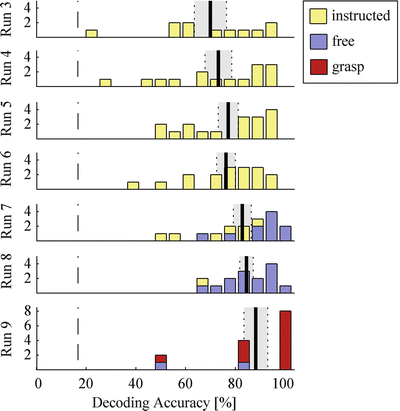
Fig. 2
Performance histograms. The ordinate indicates the number of subjects who achieved the respective decoding performance out of 19 possible percentage bins, equally spaced from 0 to 100 %. The histograms show data from different runs, chronologically ordered from top to bottom. The run modes are coded by color. Vertical dashed lines indicate the guessing level and thick solid lines indicate the average decoding accuracies over subjects. Standard error is marked grey
An established measure for the comparison of BCIs is the information transfer rate (ITR) which combines decoding accuracy and number of alternatives to a unique measure. We calculated the ITR according to the method of Wolpaw et al. [14] at 3.4–12.0 bit/min for single subjects and 8.1 bit/min on average. Note that the maximum achievable bit rate with the applied stimulation scheme is 15.5 bit/min.
For online eye movement control, we observed the subjects’ eyes on a video screen. In addition, we inspected the EOG measurements offline. Both methods confirmed that subjects followed the instruction to keep fixation.
3.2 Grasping Performance
We evaluated the execution duration of the online grasp calculation for different setups and objects. We implemented our grasping algorithm with the ability to distribute force computations to several parallel threads. Here, we permitted five threads employing a 2.8 GHz AMD Opteron 8220 SE processor. We calculated grasps of the six objects shown in Fig. 1. To assess effects of object position, we arranged the objects at different positions within the limits of our demonstrating robot’s work space. Each object was placed once at each of the positions depicted in Fig. 1. The time needed to plan the trajectory and execute the grasp until reaching force closure is listed in Table 2 for each object/position combination. Calculation times ranged from 11 to 72.6 s depending on the object and the position. The diagonal of Table 2 represents the actual object/position setup during our experiment.
Table 2
Duration of grasp planning calculation for all object/position combinations in seconds


