Spatiotemporal Pattern Classification of the Stimuli on Different Fingers

(1)

$\displaystyle{ A_{j}(t) = \sqrt{v_{j }^{2 }(t) + u_{j }^{2 }(t)}, }$

(2)

$\displaystyle{ \phi _{j} = a\tan \left (\frac{v_{j}(t)} {u_{j}(t)}\right ),j = 1,\ldots,64. }$

(3)

Spatial structure of the analytic phase was fitted to a cone surface due to the similarity [8], and the phase cones constitute the PM patterns. The 8 × 8 phase surface at each time sample was fitted to in Eq. 4.

$\displaystyle{ \phi (t) =\phi _{0}(t) +\gamma (t)\sqrt{[x_{i } - x_{0 } ]^{2 } + [y_{i } - y_{0 } ]^{2}}. }$

(4)

Where ϕ(t) was the vertical offset of the cone apex, x _j, y _jwas the cone apex, x ₀, y ₀ was the center of the electrode array, and γ(t) was the slope of the cone.

Stable frames were obtained by applying technical criteria and physiological criteria to these parameters of phase cones and frames. There was detailed description of the criteria in [8–10]. Analytic power, which was square of analytic amplitude, specified the spatial pattern of amplitude modulation. After analytic power was subtracted by spatial ensemble average and normalized by dividing temporal standard deviation, 64 × 1 feature vector of each stable frame was extracted as root mean square of values over all time samples of the stable frame on each channel. Each finger was stimulated for 40 times in one experiment so that each feature matrix was 64 × 40.

Feature vectors were classified by a three-layer BP network with optimized parameters. There were nine neurons on the hidden layer and function traingda() in MATLAB was implemented as learning algorithm. The training set consisted of half of the samples and the other half were used as the testing set. They were then switched for crosscheck. The final result was computing the average for results of test and crosscheck. KIII model, a bionic olfactory system model, has many dynamic behaviors such as limit cycle, quasi-periodic oscillation and chaos [11, 12]. It has been widely applied to pattern recognition due to its reliable pattern learning. Another classification algorithm for comparison was using KIII model to preprocess the feature vectors, afterwards, the output be classified by the same BP network applied before. Four samples of each class were used to train KIII model twice for pattern learning and others were classified by BP after preprocessed. Sixteen samples were selected as training set and 20 samples as testing set in each class for BP network.

3 Results

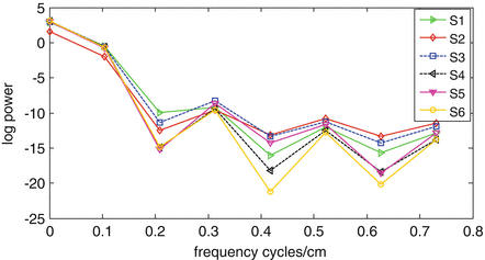
It was necessary to remove spatial noise as the high-density EEGs were measured locally (Fig. 1). The phase surfaces were much smoother with preprocessing of the appropriate low-pass spatial filtering than those with no spatial filtering preprocessing (Fig. 2).

Fig. 1

Mean spatial power spectral density for each subject

Fig. 2

Spatial phase structure obtained (a) before spatial filtering and (b) after spatial filtering

Optimized preprocessing could improve classification rate. Optimal bandwidth of the temporal filter was selected repeatedly as 15–24 Hz and cutoff frequency of the spatial filter was 0.43 cycles/cm to get high classification rate.

The patterns of the stimuli on index finger and little finger of right hand were recognized only in beta range in this study as well as index finger and ring finger of right hand with shorter distance. Patterns in gamma band could not be classified.

Only gold members can continue reading. Log In or Register to continue