State of the Art and Perspectives of Ultrasound Imaging as a Human-Machine Interface

Fig. 2.1

Karl Dussik’s apparatus to generate ultrasonic waves, built in 1942 (Reproduced from [17])

In 1948, the first Congress of Ultrasound in Medicine was held in Erlangen, Germany; in 1955 the terms A-mode and B-mode ultrasound scanning (in turn, amplitude- and brightness-modes) were used for the first time, namely by John J. Wild at Cambridge. Lastly, in 1958 Ian Donald started using ultrasonic scanning as an aid to medical diagnoses in the case of an abdominal tumour; his pioneeristic result were published in Lancet [15]. Two years later, he developed the first two-dimensional ultrasonic scanner, and this is probably the point where modern ultrasound imaging is born.

Musculoskeletal ultrasonography, that is, ultrasound scanning of bones, muscles and tendons, starts in 1958 again thanks to Dussik [18] who measured the acoustic attenuation of articular and periarticular tissues. To obtain a US image of a musculoskeletal structure though, one must wait until McDonald and Leopold’s 1972 paper [34]; in which it is stated that two musculoskeletal conditions (namely, Baker’s cysts and peripheral oedema) produce two different ultrasound patterns, which can be distinguished both from each other and from a healthy condition.

This is likely to be one of the first general diagnostic statements of a musculoskeletal condition based upon ultrasound imaging.

Although the basic principle has not changed, the performances of today’s ultrasound machines are excellent under all points of view. Thanks to the blazing advancements in both piezoelectric technology, microelectronics and computer processing power, modern ultrasound machines can obtain full-resolution B-mode ultrasonic scans, that is, grey-valued images, of essentially any body structure. Current machines [28] reach temporal resolutions of up to 100 frames per second, spatial resolutions of 0.3–1 mm in the direction parallel to the transducer (the device leaning against the subject’s skin), can visualise up to 15 × 15 cm of tissue, and can be made so small that they are not bigger than a smartphone; there are examples of commercial hand-held ultrasound machines weighing 390 g with a 3. 5″ display.

2.2.2 Technological Principles of Ultrasound Imaging

A full mathematical treatment of (medical) ultrasound imaging can be found, e.g., in [12, 28]; what follows is an informal description of the physics and technology underlying medical imaging. For a more technical description of how a medical ultrasonography device works, see, e.g., [1].

With the term ultrasound it is commonly meant sound waves of frequency over 20 kHz. The propagation speed v of a sound (mechanical) wave in a physical medium depends on the mechanical characteristics of the medium itself according to the relation $v = \sqrt{\frac{B} {\rho }}$ , where B is the medium’s adiabatic bulk modulus and ρ is the medium’s density. (The adiabatic bulk modulus measures the resistance of a substance to uniform compression.) Therefore, wherever a gradient in the medium’s density or stiffness is found, v will change and so will the energy associated to the wave. The differential in energy can in general result in wave absorption, transmission and reflection; in a real situation, all three phenomena will occur to different degrees, and the phenomenon will be particularly evident each time the wave hits the boundary between two different mediums.

As a result of that, any device able to measure the reflection of a definite wave after it has travelled back and forth in a region of interest will be able to determine what boundaries the wave itself has been travelling through before being attenuated beyond recognition. In the case of ultrasound waves, this principle lies beneath the ability of some animal species such as, e.g., bats to navigate flight and to locate food sources.

Fig. 2.2

(Left) A graphical representation of how ultrasound imaging works (Reproduced from [1]); (right) a scheme of the typical linear B-mode ultrasonographic device (Reproduced from [28])

In the case of ultrasound imaging (see Fig. 2.2, left panel), an array of piezoelectric transducers is used to focus a multiplexed, synchronised set of ultrasound waves (beam) over a line lying at few centimeters’ distance from the array. Each element of the array can, in turn, be used to convert the echo(es) of the emitted wave into a voltage. By accurately timing the echoes, one can determine the nature of the medium through which the wave has propagated; in particular, the echoes form the profile of the boundaries encountered along a straight line stretching away from the transducers. This information can be plotted, forming the so-called A-mode ultrasonography.

By employing a multiplexing device (beamformer), all transducers in the array can be synchronised to gather closely spaced profiles. The net result is a two-dimensional representation of the section of the medium lying ahead of the array, or a so-called B-mode ultrasonography. (The array is often called the probe of the ultrasound machine, or, with a slight abuse of language, the transducer.) The intensity in the profiles, and therefore in their 2D juxtaposition (image) denotes rapid spatial variations in B and/or ρ, therefore indicating abrupt changes of medium – interfaces. Figure 2.2 (right panel) shows a scheme of the typical B-mode ultrasonographic device: the ultrasound beam generated by the transmit beamformer sweeps the tissues of interest, generating reflections at each point in space where an interface between two tissues is found. Corresponding reflections are captured by the transducers and converted to a grey-valued image by a receive beamformer coupled with a time-delay compensation device. As a result, “ridges” in the image denote tissue interfaces.

The frequency selected for the ultrasound waves must be tuned, within a reasonable range, according to the tissue under examination and the required focus depth and depth of field; typically, wave frequencies are between 2 and 18 MHz.

2.2.3 Ultrasound Imaging in Rehabilitation Robotics

In rehabilitation robotics, a complex robotic artifact must be somehow interfaced with a disabled human subject. Depending on the task the subject requires and on which functionalities the robotic artifact provides, the rehabilitation engineer must figure out how to let the subject control the artifact to the best possible extent – the main issues here are those of reliability, dexterity and practical usability. An HMI lies therefore at the core of such a man-machine integration, and must be targeted on the patient’s needs and abilities.

In particular, one must figure out, first of all, what kind of signals best suit the target application. The signals must be recognisable into stable and repeatable patterns, and must be produced by the subject with a reasonable effort, both physical and cognitive. Such patterns must then be converted into (feed-forward) control signals, i.e., motion or force commands for the robotic artifact. One early example of such a successful HMI is sEMG, initially developed as a diagnostic tool for assessing peripheral neural disorders and muscular conditions; from the 1960s on then, it was applied to control single-degree-of-freedom hand prosthesis, and its use has then progressed towards lower- and upper-limb self-powered prostheses [37]. More or less at the same time, advanced pattern recognition techniques started being used to convert the sEMG signal patterns into control signals, whenever the dexterity of the prosthesis called for a finer detection of the subject’s intentions [14, 19, 35].

The wealth of information delivered by medical ultrasound imaging, therefore, calls for the exploration of its use as a novel HMI in this field. The idea of applying machine learning techniques to ultrasound images in general is not new. Recent examples include, e.g., the recognition of skin cancer [30], tumor segmentation [50] and anatomical landmarks detection in the foetus [39]. But, as far rehabilitation robotics is concerned, the literature is scarce. To the best of our knowledge, at the time of writing the only application is that of 3D ultrasound imaging to the visualisation of residual lower limbs and to assess the ergonomy of lower-limb prostheses [16, 38].

2.3 Sonomyography

The first real use of US imaging as an HMI appears in 2006 and is due to Yong-Ping Zheng et al. [51]. The associated technique is called sonomyography. The authors focus on the large extensor muscle of the forearm, M. Extensor Carpi Radialis, and perform a wrist flexion/extension experiment on six intact subjects and three trans-radial amputees. In the study, two rectangular blocks are used to track the upper and lower boundaries of the muscle; tracking is enforced using a custom tracking algorithm based upon 2D cross-correlation between subsequent frames. The estimated muscle thickness is the distance between the centres of the two blocks. See Fig. 2.3.

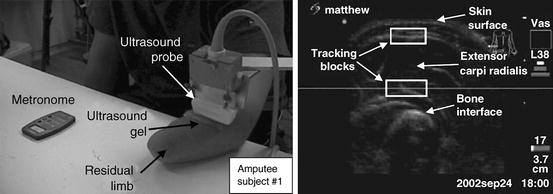
Fig. 2.3

Determining the wrist flexion angle via ultrasound imaging. (Left) The setup; (right) a typical US image (Reproduced from [51])

The wrist flexion angle is determined using a motion tracking system and four markers placed on the subject’s wrist and dorsum of the hand; in the case of the amputees, the subjects were asked to imagine flexing and extending the imaginary wrist while listening to an auditory cue (metronome). The correlation coefficient between the estimated muscle width and the wrist flexion angle is evaluated, showing high correlation in the cases of the intact subjects (linear regression average R ² coefficient 0.875). A qualitative analysis of the results for the amputees is promising.

Extensive work on the same topic follows in a series of studies. In [26] high correlation is shown among wrist angle, sonomyography and the root-mean-square of the sEMG signal, which is well-known to be quasi-linearly related to the force exerted by a muscle [14]. The proposed approach is therefore validated by comparison with a standard technique and with the ground truth. In [42] a new algorithm is presented which further improves the previous results; lastly, in [23] a successful discrete tracking task controlled by sonomyography is presented. The subject pool is this time sensibly larger (16 intact subjects). As a follow-up, the feasibility of using sonomoygraphy to control a hand prosthesis has been demonstrated [10, 11, 42], but still limited to wrist flexion and extension. Attempts have been made to improve the estimation of wrist angle from sonomyography using support vector machine and artificial neural network models [24, 47].

More recently, sonomyography has been successfully extended to elbow flexion/extension, wrist rotation, knee flexion/extension and ankle rotation [52]. Lastly, and this is probably the most interesting result so far [24], the approach is extended to A-mode ultrasonography: a wearable, single ultrasound transducer is used to determine the wrist flexion angle via a support vector machine [3, 13]. A-mode ultrasonography is enforced by means of commercially available single ultrasound transducers applied on the subject’s skin, much like sEMG electrodes. This opens up the possibility of miniaturising the sonomyography hardware and make it wearable. The issue of signal generation and conditioning is still open, though.

In the above-mentioned corpus of research, the authors have never considered more than one feature at the same time. This restricted focus is probably motivated by the diversity and complexity of the changes in US images as joint positions change: the single identified feature is related to a precise anatomical change, a relation which would be quite hard to assess in the general case. It is likely that a more general treatment in that case would require a detailed model of the kinematics of the human forearm, plus a detailed model of the changes in the projected US image as the hand joints move – a task which seems overtly complex. The only attempt so far at modelling finger positions appears in [43, 44], where significant differences among optical flow computations for finger flexion movements are reported and classified.

2.4 Ultrasound Imaging as a Realistic HMI

The only other attempt at establishing US imaging as an HMI, as far as we know, is that carried on in our own group. In particular, with respect to sonomyography, this approach does not rely on anatomical features of the forearm (as visualised in the ultrasonic images), but rather considers the images as a global representation of the activity going on in the musculoskeletal structure, as a human subject performs movement or force patterns with the hand. (This approach cannot therefore be consistently called “sonomyography”, as the targeted structures are not restricted to muscles, but rather all organs are considered, i.e., veins and arteries, bones, nerves, connective and fat tissue, etc.)

2.4.1 Ultrasound Images of the Forearm

In [5, 49] the first qualitative/quantitative analysis of the ultrasonographic images of the human forearm, with respect to the finger movements, was carried out. Extensive qualitative trials were performed, i.e., live ultrasound images of sections of the human forearm were considered, while the subject would turn the wrist and/or flex the fingers, both singularly and jointly. An example is visible in Fig. 2.4.

Fig. 2.4

(Left) A typical ultrasound image obtained during the qualitative analysis carried on in [5]. The ulna is clearly visible in the bottom-left corner, while the flexor muscles and tendons are seen in the upper part. (Right) A graphical representation of the human forearm and hand (right forearm; dorsal side up). The transducer is placed onto the ventral side; planes A and B correspond to the sections of the forearm targeted by the analysis

One first result was that clearly, subsequent images related to each other in non-trivial ways. Human motion is in general enacted by contracting the muscles. When a muscle contracts, its length reduces but its mass must obviously remain constant; as a consequence, the muscle swells, mainly in the region where most muscle fibers are concentrated. This region, colloquially referred to as the muscle belly, expands in the directions orthogonal to the muscle axis; at the same time, the other organs in the forearm must accordingly shift around – this includes the bones, nerves, tendons and connective/fat tissue.

In the experiment, the ultrasound probe was held orthogonal to the forearm main axis, visually resulting in a complex set of motions: muscle sections (elliptical structures in the images) would shrink and expand; sometimes the muscle-muscle and muscle-tendon boundaries would disappear and reappear; and meanwhile, all other structures around would move in essentially unpredictable ways. It was clear that the deformations seen in the images could not easily be described in terms of simple primitives, such as, e.g., rotations, translations and contractions/expansions. Only very few simple features could have been explicitly targeted using anatomical knowledge, as it had been done in sonomyography; but as well, anatomy varies across subjects, which would have hampered the general applicability of the approach.

At the same time, it was apparent that whatever force the subject exerted (the three degrees of freedom of the wrist, the motion of single fingers down to the distal joints, etc.) was related point-to-point to the images. Muscular forces relate to torques at the joints, which in turn relate to measurable forces at the end effectors, for example at the fingertips. In the visual inspection there was no hysteresis effect, and each single dynamic configuration of the musculoskeletal structures under the skin would clearly correspond to a different image. This was the case both when the fingers would freely move and when they would apply force against a rigid surface or an object to be grasped. (Actually, that hinted at the fact that free movement actually represents the application of small forces, that is, those needed to counter the intrinsic impedance of the musculoskeletal structures.)

One direct consequence of this is that wrist and finger positions and forces could clearly be directly related point by point to each single image. This hinted at the possibility of using spatial features of the ultrasound images to predict the hand kinematic configuration (rather than, e.g., the optical flow or other features involving the time derivative of the images). This would have the advantage of being independent of the speed with which forces were applied.

Another very interesting characteristic of the forearm US images was that changes related to the hand/forearm kinematic configuration were almost totally local; e.g., it was tested that when the subject flexed the little finger, deformations would happen almost only in a certain region of the images; the region is loosely determined by the underlying anatomy. If, e.g., the US transducer was placed on the ventral side of the wrist, orthogonal to the axis of the forearm, then the action would be limited almost exclusively to the tendon leading out of the large flexor muscle (M. Flexor Digitorum Superficialis) controlling the little finger. The tendon pulls backwards and forwards parallel to the forearm axis, and appears as an elliptic structure growing and shrinking in a corner of the images. This further suggested the use of local spatial features of the images.

2.4.2 Relating US Images and Finger Angles/Forces

In the above-mentioned paper and in the subsequent [8], it was established that linear local spatial first-order approximations of the grey levels are linearly related to the angles at the metacarpophalangeal joints of the hand, leading to an effective prediction of the finger positions. More in detail, a uniform grid of N interest points, $p_{i} = (x_{i},y_{i}),i = 1,\ldots,N$ , was considered; a circular region of interest (ROI) of radius r > 0, centered around each interest point, would then be determined:

$\displaystyle{\mbox{ ROI}_{i} =\{ (x,y): (x - x_{i})^{2} + (y - y_{ i})^{2} \leq r^{2}\}}$

Lastly, for each ROI, a local spatial first-order approximation of the grey values of its pixels G(x, y) was evaluated:

$\displaystyle{G(x,y)\ \approx \ \alpha _{i}(x_{i} - x) +\beta _{i}(y_{i} - y) +\gamma _{i}}$

for all (x, y) ∈ ROI_i. Intuitively, α _idenotes the mean image gradient along the x direction (rows of the image), β _iis the same value along the y (columns) direction, and γ _iis an offset. Figure 2.5 shows the grid of points and graphically illustrates the meaning of these features.

Fig. 2.5

(Above) A graphical representation of the meaning of the spatial features α _i, β _i, γ _i; (below) the grid of interest points, as laid out on a typical US image (Reproduced from [49])

The above remark about the locality of the image changes is reflected in the changes in the feature values: Fig. 2.6 shows a correlation diagram, obtained by considering the Pearson correlation coefficient between the average of $\alpha _{i},\beta _{i},\gamma _{i}$ and values of the sensor of the little finger of a dataglove (experiment reported in [8]). As is apparent from the figure, the movement of the little finger is strongly correlated to the feature values in the upper-left corner of the images.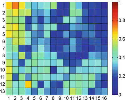

Fig. 2.6

Correlation diagram of the movement of the little finger. Each entry in the matrix denotes, for each region of interest i, the Pearson correlation coefficient between $\frac{\alpha _{i}+\beta _{i}+\gamma _{i}} {3}$ and the dataglove sensor values obtained while moving the little finger