Statistics and the Design of Experiments and Surveys
Graham Dunn
Introduction
Research into mental illness uses a much wider variety of statistical methods than those familiar to a typical medical statistician. In many ways there is more similarity to the statistical toolbox of the sociologist or educationalist. It would be a pointless exercise to try to describe this variety here but, instead, we shall cover a few areas that are especially characteristic of psychiatry. The first and perhaps the most obvious is the problem of measurement. Measurement reliability and its estimation are discussed in the next section. Misclassification errors are a concern of the third section, a major part of which is concerned with the estimation of prevalence through the use of fallible screening questionnaires. This is followed by a discussion of both measurement error and misclassification error in the context of modelling patterns of risk.
Another major concern is the presence of missing data. Although this is common to all areas of medical research, it is of particular interest to the psychiatric epidemiologist because there is a long tradition (since the early 1970s) of introducing missing data by design. Here we are thinking of two-phase or double sampling (often confusingly called two-stage sampling by psychiatrists and other clinical research workers). In this design a first-phase sample are all given a screen questionnaire. They are then stratified on the basis of the results of the screen (usually, but not necessarily, using two strata—likely cases and likely non-cases) and subsampled for a second-phase diagnostic interview. This is the major topic of the third section.
If we are interested in modelling patterns of risk, however, we are not usually merely interested in describing patterns of association. Typically we want to know if genetic or environmental exposures have a causal effect on the development of illness. Similarly, a clinician is concerned with answers to the question ‘What is the causal effect of treatment on outcome?’ How do we define a causal effect? How do we measure or estimate it? How do we design studies in order that we can get a valid estimate of a causal effect of treatment? Here we are concerned with the design and analysis of randomized controlled trials (RCTs). This is the focus of the fourth section of the present chapter.
Finally, at the end of this chapter pointers are given to where the interested reader might find other relevant and useful material on psychiatric statistics.
Reliability of instruments
In this section we consider two questions:
What is meant by ‘reliability’?
How do we estimate reliabilities?
Models and definitions
Most clinicians have an intuitive idea of what the concept of reliability means, and that being able to demonstrate that one’s measuring instruments have high reliability is a good thing. Reliability concerns the consistency of repeated measurements, where the repetitions might be repeated interviews by the same interviewer, alternative ratings of the same interview (as a video recording) by different raters, alternative forms or repeated administration of a questionnaire, or even different subscales of a single questionnaire, and so on. One learns from elementary texts that reliability is estimated by a correlation coefficient (in the case of a quantitative rating) or a kappa (κ) or weighted κ statistic (in the case of a qualitative judgement such as a diagnosis). Rarely are clinicians aware of either the formal definition of reliability or of its estimation through the use of various forms of intraclass correlation coefficient rho (ρ).
First consider a quantitative measurement X. We start with the assumption that it is fallible and that it is the sum of two components: the ‘truth’ T and ‘error’ E. If T and E are statistically independent (uncorrelated), then it can be shown that
where Var(X) is the variance of X (i.e. the square of its standard deviation), and so on. The reliability &Rgr;x of X is defined as the proportion of the total variability of X (i.e. Var(X)) that is explained by the variability of the true scores (i.e. Var(T)):
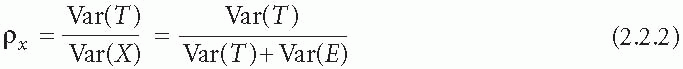
This ratio will approach zero as the variability of the measurement errors increases compared with that of the truth. Alternatively, it will approach one as the variability of the errors decreases. The standard deviation of the measurement errors (i.e. the square root of Var(E)) is usually known as the instrument’s standard error of measurement. Note that reliability is not a fixed characteristic of
an instrument, even when its standard error of measurement (i.e. its precision) is fixed. When the instrument is used on a population that is relatively homogeneous (low values of Var(T)), it will have a relatively low reliability. However, as Var(T) increases then so does the instrument’s reliability. In many ways the standard error of measurement is a much more useful summary of an instrument’s performance, but one should always bear in mind that it too might vary from one population to another—a possibility that must be carefully checked by both the developers and users of the instrument.
an instrument, even when its standard error of measurement (i.e. its precision) is fixed. When the instrument is used on a population that is relatively homogeneous (low values of Var(T)), it will have a relatively low reliability. However, as Var(T) increases then so does the instrument’s reliability. In many ways the standard error of measurement is a much more useful summary of an instrument’s performance, but one should always bear in mind that it too might vary from one population to another—a possibility that must be carefully checked by both the developers and users of the instrument.
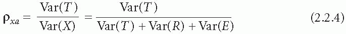
Now let us complicate matters slightly. Suppose that a rating depends not only on the subject’s so-called true score T and random measurement error E, but also on the identity R, say, of the interviewer or rater R. That is, each rater has his or her own characteristic bias (constant from assessment to another) and the biases can be thought of as varying randomly from one rater to another. Again, assuming statistical independence, we can show that, if X = T + R + E, then
But what is the instrument’s reliability? It depends. If subjects in a survey or experiment, for example, are each going to be assessed by a rater randomly selected from a large pool of possible raters, then
However, if only a single rater is to be used for all subjects in the proposed study, there will be no variation due to the rater and the reliability now becomes
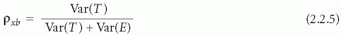
Of course, Pxb > Pxa. Again, the value of the instrument’s reliability depends on the context of its use. This is the essence of generalizability theory.(1) The three versions of p given above are all intraclass correlation coefficients and are also examples of what generalizability theorists refer to as generalizability coefficients.
Designs
Now consider two simple designs for reliability (generalizability) studies. The first involves each subject of the study being independently assessed by two (or more) raters but that the raters for any given subject have been randomly selected from a very large pool of potential raters. The second design again involves each subject of the study being independently assessed by two (or more) raters, but in this case the raters are the same for all subjects. Equations (2.2.1) and (2.2.2) are relevant to the analysis of data arising from the first design, whilst eqns (2.2.3, 2.2.4 and 2.2.5) are relevant to the analysis of data from the second design.
Estimation of ρ and κ from ANOVA tables
When we come to analyse the data it is usually appropriate to carry out an analysis of variance (ANOVA). For the first design we carry out a one-way ANOVA (X by subject) and for the second we perform a two-way ANOVA (X by rater and subject). In the latter case we assume that there is no subject by rater interaction and accordingly constrain the corresponding sum of squares to be zero. We assume that readers are reasonably familiar with an analysis of variance table. Each subject has been assessed by, say, k raters. The one-way ANOVA yields a mean square for between-subjects variation (BMS) and a mean square for within-subjects variation (WMS). WMS is an estimate of Var(E) in eqn. (2.2.1). Therefore, the square root of WMS provides an estimate of the instrument’s standard error of measurement. The corresponding estimate of &Rgr;x is given by
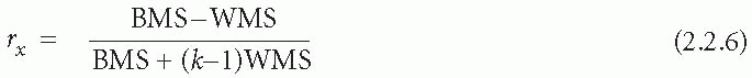
where rx is used to represent the estimate of &Rgr;x rather than the true, but unknown, value. In the case of k = 2, rx becomes

In the slightly more complex two-way ANOVA, the ANOVA table provides values of mean squares for subjects or patients (PMS), raters (RMS), and error (EMS). We shall not concentrate on the details of estimation of the components of eqn. (2.2.3) (see Fleiss(2) or Streiner and Norman(3)) but simply note that &Rgr;xa is estimated by

where n is the number of subjects (patients) in the study.
In reporting the results of a reliability study, it is important that investigators give some idea of the precision of their estimates of reliability, for example by giving an appropriate standard error or, even better, an appropriate confidence interval. The subject is beyond the scope of this chapter, however, and the interested reader is referred to Fleiss(2) or Dunn(4) for further illumination.
Finally, what about qualitative measures? We shall not discuss the estimation and interpretation of κ in any detail here but simply point out that for a binary (yes/no) measure one can also carry out a two-way analysis of variance (but ignore any significance tests since they are not valid for binary data) and estimate rxa as above. In large samples rxa is equivalent to κ.(3) A corollary of this is that K is another form of reliability coefficient and, like any of the reliability coefficients described above, will vary from one population to another (i.e. it is dependent on the prevalence of the symptom or characteristic being assessed).
Prevalence estimation
Following Dunn and Everitt,(5) we ask the following questions of a survey report.
Do the authors clearly define the sampled population?
Do the authors discuss similarities and possible differences between their sampled population and the stated target population?
Do the authors report what sampling mechanism has been used?
Is the sampling mechanism random? If not, why not?
Exactly what sort of random sampling mechanism has been used?
Do the methods of data analysis make allowances for the sampling mechanism used?
Of course, it is vital that what counts as a case should be explained in absolute detail, including the method of eliciting symptoms (e.g. structured interview schedule), screening items, additional impairment criteria, and so on, as well as operational criteria or algorithms used in making a diagnosis. In the following we concentrate on the statistical issues. First, we consider survey design (and the associated sampling mechanisms), and then we move on to discuss the implications of design for the subsequent analysis of the results.
Survey design
Here we are concerned with the estimation of a simple proportion (or percentage). We calculate this proportion using data from the sample and use it to infer the corresponding proportion in the underlying population. One vital component of this process is to ensure that the sampled population from which we have drawn our subjects is as close as possible to that of the target population about which we want to draw conclusions. We also require the sample to be drawn from the sample population in an objective and unbiased way. The best way of achieving this is through some sort of random sampling mechanism. Random sampling implies that whether or not a subject finishes up in the sample is determined by chance. Shuffling and dealing a hand of playing cards is an example of a random selection process called simple random sampling. Here every possible hand of, say, five cards has the same probability of occurring as any other. If we can list all possible samples of a fixed size, then simple random sampling implies that they all have the same probability of finishing up in our survey. It also implies that each possible subject has the same probability of being selected. But note that the latter condition is not sufficient to define a simple random sample. In a systematic random sample, for example, we have a list of possible people to select (the sampling frame) and we simply select one of the first 10 (say) subjects at random and then systematically select every tenth subject from then on. All subjects have the same probability of selection, but there are many samples which are impossible to draw using this mechanism. For example, we can select either subject 2 or subject 3 with the same probability (1/10), but it is impossible to draw a sample which contains both.
What other forms of random sampling mechanisms might be used? Perhaps the most common is a stratified random sample. Here we divide our sampled population into mutually exclusive groups or strata (e.g. men and women, or five separate age groups). Having chosen the strata, we proceed, for example, to take a separate simple random sample from each. The proportion of subjects sampled from each of the strata (i.e. the sampling fraction) might be constant across all strata (ensuring that the overall sample has the same composition as the original population), or we might decide that one or more strata (e.g. the elderly) might have a higher representation. Another commonly used sampling mechanism is multistage cluster sampling. For example, in a national prevalence survey we might chose first to sample health regions or districts, then to sample post codes within the districts, and finally to select patients randomly from each selected post code. (See Kessler(6) and Jenkins et al.(7) for discussions of complex multistage surveys of psychiatric morbidity.)
One particular design that has been used quite often in surveys designed to estimate the prevalence of psychiatric disorders is called two-phase or double sampling. Psychiatrists frequently refer to this as two-stage sampling. This is unfortunate, since it confuses the two-phase design with simple forms of cluster sampling in which the first-stage involves drawing a random sample of clusters and the second-stage a random sample of subjects from within each of the clusters. In two-phase sampling, however, we first draw a preliminary sample (which may be simple, stratified, and/or clustered) and then administer a first-phase screening questionnaire such as the General Health Questionnaire (see Chapter 1.8.1). On the basis of the screen results we then stratify the first-phase sample. Note that we are not restricted to two strata (likely cases versus the rest), although this is perhaps the most common form of the design. We then draw a second-phase sample from each of the first-phase strata and proceed to give these subjects a definitive psychiatric assessment. The point of this design is that we do not waste expensive resources interviewing large numbers of subjects who not appear (on the basis of the first-phase screen) to have any problems. Accordingly, the sampling fractions usually differ across the first-phase strata. However, it is vital that each of the first-phase strata have a reasonable representation in the second-phase, and it is particularly important that all of the first-phase strata provide some second-phase subjects. The reader is referred to Pickles and Dunn(8) for further discussion of design issues in two-phase sampling (including discussion of whether it is worth the bother).
Related posts:


Stay updated, free articles. Join our Telegram channel

Full access? Get Clinical Tree


