Fig. 7.1
Magnetic resonance images of a 24-week-old foetus. From Anblagan et al. (unpublished observation)
The same scanner can be used for acquiring different types of images by changing the exact parameters of an MR “scan”: the temporal sequence of radiofrequency (RF) pulses, gradients and read-outs (see Sect. 7.2 for basic principles). Thus, in one MRI session, we can run several scans to assess a number of functional and structural properties of the human brain (Table 7.1).
Table 7.1
An example of a 60-min MR protocol enabling one to characterize a number of structural and functional properties of the human brain
MRI sequence | Time (min) | Structure and physiology |
|---|---|---|
T1-weighted | 10 | Volumes, thickness, folding, shape, tissue density |
T2-weighted | 4 | White-matter hyperintensities (number, volume, location) |
Diffusion tensor imaging | 12 | Fractional anisotropy, mean diffusivity, track delineation |
Magnetization transfer | 8 | Myelination index |
Arterial spin labelling | 5 | Perfusion |
Resting-state functional | 8 | Spontaneous cerebral networks; functional connectivity |
Paradigm-based functional | 6–10 | Brain response associated with specific stimuli/tasks; functional connectivity |
Most of these measurements are made evenly throughout the brain—one measurement (or value) per “voxel”.2 Depending on the spatial resolution of the 3D image, thousands of measurements are acquired simultaneously during each scan. Thus, for example, a typical T1-weighted image of the head contains ~10 million voxels (1 × 1 × 1 mm in size), of which about 1.5 million will be inside the brain. But not all MR protocols cover the brain in such an even and unbiased fashion. One notable exception to this desirable feature is that of a paradigm-based functional MRI (fMRI). Although the whole brain is being scanned, we can draw inferences about brain function only from the measurements acquired in the parts of the brain that are engaged by the paradigm (see Sect. 7.4 for details).
As indicated in Table 7.1, MR allows us to assess a large number of structural properties and, unlike fMRI, do so in an unbiased and highly reliable way throughout the brain. Nonetheless, two important issues should be kept in mind when interpreting these measurements: (1) neurobiology underlying the MR metrics and (2) directionality of the brain-behaviour relationships.
First, mapping of the various MR-derived metrics onto the underlying neurobiology is complicated by the fact that each MR voxel contains a mix of various cellular elements (Fig. 1.5). Therefore, we cannot attribute unequivocally a particular biological process to a difference/change in an MR-derived measurement (e.g. cortical thickness) without additional evidence. Genetics may be quite useful in this context. For example, moderating effects of functional polymorphisms in the gene for vascular endothelial growth factor (VEGF) may support one particular interpretation of the observed difference/change in cortical thickness, namely that of differential vascularization. But—of course—only a combination of in vivo (MRI) and ex vivo (e.g. immunohistochemistry) studies in experimental animals can provide more definite answers with regard to the biology underlying MR-based phenotypes.
Second, structure–function relationships can work in both directions: a structural change can precede a functional change and vice versa. It is quite likely, for example, that prenatal and early post-natal events would have significant (and direct) impact on brain growth, with direct consequences on brain function and mental health later in life. We have shown, for example, that an exposure to maternal cigarettes smoking during pregnancy in female offspring (i.e. daughters of the smoking mothers) with a particular genetic variant is associated with a significant (~10 %) reduction in the overall cortical area (Fig. 7.2), possibly through an accentuated apoptosis of progenitor cells during embryogenesis (Paus et al. 2012). In the long term, this reduction in “brain reserve” might—for example—increase the risk of these individuals for dementia.
Fig. 7.2
Brain volume, cortical area and cortical folding in female offspring exposed (left) and non-exposed (right) to maternal cigarette smoking during pregnancy, as a function of KCTD8 genotype (rs716890). From Paus et al. (2012)
On the other hand, a functional engagement of a given brain region may—over time—lead to subtle structural changes detectable with MRI. A classical example of this function-to-structure path, revealed with structural MRI, is that of a repeated practice of juggling: an increase in regional amount of grey matter (GM) in a cortical area engaged by visual motion, after 3 months of learning how to juggle three balls (Fig. 7.3). Note, however, that we can only speculate about the neurobiology (dendrites, vascularization, glia) underlying this change.
Overall, MRI is a highly versatile tool that allows us to quantify a large number of functional and structural brain phenotypes in both global and regional manner. Let us now review the basic principles of this technology.
7.2 MRI: Basic Principles
Nuclei that have an odd number of nucleons (protons and neutrons) possess both a magnetic moment and angular momentum (or spin). In the presence of an external magnetic field, such nuclei “line up” with the main magnetic field and precess (or spin) around their axis at a rate proportional to the strength of the magnetic field, emitting electromagnetic energy as they do. The hydrogen atom contains only a single proton and therefore precesses when exposed to a magnetic field.
In the majority of MR imaging studies, precessing nuclei of hydrogen associated with water and fat is the source of the signal. The signal is generated and measured in the following way. First, the person is exposed to a large static magnetic field (B0) that aligns hydrogen nuclei along the direction of the applied field. In clinical scanners, the strength of B0 is most often 1.5 Tesla;3 B0 is oriented horizontally, pointing from head to toe along the long axis of the cylindrical magnet. Second, a pulse of electromagnetic energy is applied at a specific RF, with an RF coil placed around (or near) the head. This RF is the same as the precession frequency of the imaged nuclei at a given strength of B0. 4 The RF pulse rotates the precessing nuclei away from their axes, thus allowing one to measure, with a receiver coil, the time it takes for the nuclei to “relax” back to their original position pointing along B0. The spatial origin of the signal is determined using subtle, position-related changes in B0 induced by gradient coils.5
7.2.1 MR Contrast in Images of Brain Structure
As shown in Table 7.1, the most common MR sequences used to characterize brain structure are T1- and T2-weighted images, DTI and MTR. We will review these in turn (for a more detailed overview of MR sequences, see Roberts and Mikulis 2007).
Contrast in structural T1- and T2-weighted MR images is based on local differences in proton density6 and on the following two relaxation times: (1) longitudinal relaxation time (T1) and (2) transverse relaxation time (T2) (Fig. 7.4).
Fig. 7.4
Longitudinal (T1) and transverse (T2) relaxations times. Radio-frequency (RF) excitations are applied with a repetition time, with each excitation producing a magnetic resonance signal (Mxy; precession) that decays exponentially with a time constant T2 (right panel). Between excitations, the magnetization (Mz) also returns to its equilibrium state, pointing along the direction of the main magnetic field, with a time constant T1 (left panel). By manipulating the TR (repetition time) and TE (time-to-echo), the relative contributions of T1 and T2 can be manipulated to produce T1- and T2-weighted images. If the effects of both T1 and T2 are minimized (long TR and short TE), the remaining contrast is simply the proton density weighted. From Paus et al. (2001)
Thus, longitudinal (T1) relaxation time represents an exponential recovery of the total magnetization over time. In a complex manner, it depends on the local structural pattern (lattice)7 assumed by the hydrogen nuclei; in the brain, the more structured the tissue, the shorter T1. Transverse (T2) reflects the local “dephasing” rate for precessing nuclei8 due to local magnetic-field non-homogeneities, with a concomitant decay of the total MR signal; in the brain, the more structured the tissues, the more rapid the dephasing and hence, the shorter the T2.
Quantitative measurements of T1 and T2 relaxation times are not taken frequently, however (see Deoni et al. 2008 for a method suitable for a rapid voxel-wise measurement of T1 and T2 times). In the majority of MR studies, some combinations of T1- and/or T2-weighted images are acquired instead (Text Box 7.1).
Text Box 7.1. Acquisition of T1- and T2-weighted images
In these acquisitions, the MR signal is repeatedly measured (with a repetition time, TR) at one time point (time-to-echo, TE) after the application of each RF pulse. Local differences in relaxation times are reflected in the image contrast simply because, at a given TR/TE combination, the MR signal has already recovered (T1) or decayed (T2) to a greater extent in regions with short T1 (or T2) and vice versa. For this reason, brain tissue with a short T1 white matter (WM) appears bright on T1-weighted images; the signal has “already recovered” (Fig. 7.4, left). In contrast, tissue with a long T2 (GM) is bright on T2-weighted images; the signal has “not yet decayed” (Fig. 7.4, right).
While proton density reflects the amount of signal-emitting nuclei (i.e. protons) present in the tissue, relaxation times, and therefore tissue “brightness” on T1- and T2-weighted images, depend on a variety of biological and structural properties of the brain tissue. Water content is one of the most important influences on T1 in the brain: the more water there is in a given tissue compartment, the longer T1—and the lower the signal on a typical T1-weighted image—will be in that compartment. In the adult brain, T1 is the longest in cerebrospinal fluid (CSF), intermediate in GM and the shortest in WM. Lipid content in WM may also influence T1, through magnetic interactions with hydrogen nuclei of the lipids, which are hydrophobic. Iron content is another important influence, primarily by changing local magnetic non-homogeneities: the higher the iron content, the shorter the T2. Finally, the anatomical arrangement of axons may influence the amount of interstitial water and, in turn, T1 values; more tightly bundled axons would have shorter T1 and therefore appear brighter on T1-weighted images.
The introduction of diffusion tensor imaging (DTI) in the mid-1990s opened up new avenues for in vivo studies of white-matter microstructure (Le Bihan and Basser 1995). This imaging technique allows one to estimate several parameters of water diffusion, such as mean diffusivity (MD) and fractional anisotropy (FA), in the live brain. The latter parameter reflects the degree of water-diffusion directionality; voxels containing water that moves predominantly along a single direction have higher FA. In WM, FA is believed to depend on the microstructural features of fibre tracts, including the relative alignment of individual axons, how tightly they are packed (which affects the amount of interstitial water; see above), myelin content and axon calibre. Note that the hypothetical differences in myelination are perhaps too hastily considered as an explanation for (group, age) differences in FA, to the exclusion of other possible factors (see Fig. 7.5). In most DTI studies, the signal is coming from the movement of water in the extracellular space, complicating the interpretations of the underlying neurobiology (reviewed in Paus 2010). An interesting alternative is to measure intracellular movement of a metabolite, such as N-acethyl-aspartate, inside the axon. This can be achieved with so-called diffusion tensor spectroscopy (DTS; Upadhyay et al. 2008). Due to the high time requirements of DTS, however, this technique is not suitable—at present—for large population-based imaging studies.
Fig. 7.5
Using the short T2-component signal to estimate myelin-water fraction, Mädler et al. (2008) found a significant correlation between this measure of myelin content and FA across different brain regions within the same individual (1.5T: r2 = 0.39) but not across individuals within the same region. From Mädler et al. (2008)
Finally, magnetization transfer (MT) imaging is another MR technique employed in studies of the structural properties of WM.9 Contrast in MT images reflects the interaction between free water and water bound to macromolecules (McGowan 1999). The macromolecules of myelin are the dominant source of the MT signal in WM (Kucharczyk et al. 1994). Post-mortem studies revealed a significant positive correlation between myelin content and MTR (Schmierer et al. 2004, 2008). The fastest way to acquire MT data is to use a dual acquisition, with and without a MT saturation pulse. MTR images are calculated as the percent signal change between the two acquisitions (Pike 1996). Mean MTR values, subsequently, can be summed across all white-matter voxels constituting, for example, the four lobes of the brain.
7.2.2 MR Contrast in Images of Brain Activity
For imaging brain “activity,”10 the most common MR parameter to measure is the blood oxygenation-level-dependent (BOLD) signal detected on T2*-weighted MR images. This signal relies on the fact that neural “activation” is associated with an oversupply of oxygenated (“red”) blood to the activated brain region; consequently, small veins draining the “activated” region contain some of the “unused” oxygenated blood (“red-veins” phenomenon). In other words, the BOLD signal reflects the proportion of oxygenated (“red”) and deoxygenated (“blue”) blood in a given brain region at a given moment. Variations in the oxygenated-to-deoxygenated blood ratio provide an MR contrast. Because the deoxygenated blood contains deoxyhemoglobin, which is paramagnetic, it therefore increases local non-homogeneities. That, in turn, interferes with T2 relaxation (“dephasing”; see Sect. 7.2.1).
Now what do we measure with the BOLD signal? Although there is no dispute about the relationship between local hemodynamics and brain activity, there is still little agreement about the role various neural events play in driving the hemodynamic signal. At least two issues need to be considered when interpreting the functional significance of BOLD responses to a behavioural challenge: (1) the relative importance of neuronal firing versus synaptic activity occurring in the sampled tissue and (2) the relative contributions of excitatory and inhibitory neurotransmission.
Intuitively, a brain region requires more energy and, hence, more blood flow when neurons located in that region increase their firing rate. This notion is also conceptually attractive; if true, one would be able to take findings obtained with functional imaging of the human brain and directly correlate them with those acquired through single-unit recordings in non-human primates. Several experiments suggest, however, that firing rate is not the best predictor of local changes in hemodynamics; synaptic activity might be a better one (Text Box 7.2).
Text Box 7.2. BOLD Response: Firing Neurons or Synaptic Activity?
Using simultaneous recordings of single-unit activity, field potentials and cerebral blood flow (CBF) in the rat cerebellar cortex, Mathiesen et al. (1998) demonstrated that electrical stimulation of parallel fibres inhibited spontaneous firing of Purkinje cells located in the sampled cortex while, at the same time, it increased CBF and field potentials at the same location. On the other hand, a strong correlation (r = 0.985) was observed between postsynaptic activity, indicated by the summed field potentials and activity-dependent increases in CBF in the cerebellar cortex. Similar findings were obtained in the monkey cerebral (visual) cortex, where the local field potentials provided a better estimate of BOLD responses to visual stimulation than did multi-unit activity. While multi-unit activity increased only briefly at the onset of stimulation, the field-potential increase was sustained throughout the presence of the stimulus (Logothetis et al. 2001; Logothetis and Wandell 2004; see Fig. 7.6). In addition, Moore and colleagues showed that even subthreshold synaptic activity in the rat primary somatosensory cortex is accompanied by significant variations in hemodynamic signal (Moore et al. 1996, 1999).
Fig. 7.6
The relationship between the BOLD response (to visual stimulation) and the local field potentials (LFP) and multi-unit activity (MUA). Responses to a 24 s (upper) and 12 s (lower) stimulation are shown. The blue trace measures the LFP, the green trace measures the MUA and the red-shaded trace measures the BOLD response. The MUA signal is brief and approximately the same in both experiments. The LFP and BOLD responses co-vary with the stimulus duration. At this cortical site and in 25 % of the measurements, the LFP response matched the BOLD response, but the MUA did not. There were no instances in which the MUA matched the BOLD response but the LFP did not. From Logothetis and Wandell 2004
The second issue of interest, namely the relative contribution of excitatory and inhibitory neurotransmission to changes in local hemodynamics, is less clear cut—with one study suggesting that the former drives the signal (Text Box 7.3.).
Text Box 7.3. BOLD Response: Excitation or Inhibition?
Blockage of GABAergic transmission during electrical stimulation of parallel fibres does not appear to attenuate stimulation-induced increase in local blood flow, suggesting that the increase was primarily due to the excitatory component of the postsynaptic input (Mathiesen et al. 1998). As suggested previously (e.g. Akgören et al. 1996), a direct link between excitatory neurotransmission and local blood flow may be related to the role of nitric oxide (NO) in coupling blood flow to synaptic activity. NO is one of the signals leading to dilation of small vessels in the vicinity of “active” synapses; NO is synthesized by an enzyme called NO synthase (Northington et al. 1992; Iadecola 1993). It is known that glutamate activates NO synthase through an increase in the intracellular level of calcium and that, under physiological conditions, entry of calcium into a cell is almost exclusively linked to excitatory neurotransmission.
Overall, it is likely that changes in local hemodynamics reflect a sum of excitatory postsynaptic inputs in the sample of scanned tissue. The firing rate of “output” neurons may be related to local blood flow (Heeger et al. 2000; Rees et al. 2000), but only inasmuch as it is linked in a linear fashion to excitatory postsynaptic input. Inhibitory neurotransmission may lead to decreases in CBF, indirectly, through its presynaptic effects on postsynaptic excitation.
7.3 Structural Brain Phenotypes
Here, we provide a brief overview of the key structural phenotypes that can be derived from the MR images described in Sect. 7.2.1. (see Table 7.2 for an overview) using a number of automated image-analysis algorithms (or “pipelines”).
Table 7.2
Structural brain phenotypes
MRI sequence | Time (min) | Brain phenotypes |
|---|---|---|
3D T1-weighted | 10 | Volume, thickness, folding, shape, tissue density |
T2-weighted/FLAIR | 4 | Hyperintensities (number, volume, location) |
Diffusion tensor imaging | 12 | Fractional anisotropy, mean diffusivity, track delineation (global, regional) |
Magnetization transfer | 8 | Myelination index (global, regional) |
Traditionally, T1-weighted images have been the richest and most flexible source of data for morphometric analyses. Over the past 20 years, a number of computational pipelines have been developed by the neuroimaging community, including the Minctools from the Montreal Neurological Institute (http://www.bic.mni.mcgill.ca/ServicesSoftware/Home Page), FMRIB Software Library (FSL) from the FMRIB laboratory at the University of Oxford (http://www.fmrib.ox.ac.uk/fsl), FreeSurfer from the Martinos Centre for Biomedical Imaging (http://surfer.nmr.mgh.harvard.edu/), BrainVisa from the NeuroSpin (http://brainvisa.info), and the LONI pipeline from UCLA (http://pipeline.loni.ucla.edu/).
These pipelines enable us to extract a large number of brain features, or phenotypes (see Fig. 7.7 for an overview) in a fully automatic fashion. There are two general classes of these features: (1) Voxel- or vertex-wise11 features derived for each X, Y and Z location (e.g. grey- and white-matter “density” maps, cortical thickness, cortical folding) and (2) Volumetric measures (e.g. volumes of GM in frontal lobes, volume of the hippocampus, area of the corpus callosum). In the following text, we will describe the key computational steps involved in deriving these various features.
7.3.1 Density of Brain Tissues
First, T1-weighted images are linearly registered, from the acquisition (“native”) space to standardized stereotaxic space—such as the average ICBM/MNI-152 atlas (aligned with Talairach and Tournoux space; Evans et al. 1993). The next step involves tissue classification into GM, WM and CSF. A neural-network classifier is trained, using priors12 indicating locations that are highly likely to contain the three types of tissue (Zijdenbos et al. 2002; Cocosco et al. 2003). The tissue classification step yields three sets of binary 3D images (i.e. GM, WM and CSF). Each of the binary images can be smoothed to generate probabilistic “density” images. These maps are then used in voxel-wise analyses of age- or group-related differences in GM or WM density (see Ashburner and Friston 2000, for a methodological overview).
7.3.2 Deformation Fields
A deformation field—computed while aligning (registering) a population member to the target13—models the extent to which the anatomy of the individual differs from that of the population. Consequently, the set of all deformation fields captures the overall population variability. By comparing inter-population to intrapopulation deformations, we can identify and quantify anatomical differences in local shape between populations.14 Unlike standard volumetric approaches, this deformation-based technique can detect differences in the morphology of brain regions that do not necessarily coincide with manually defined structures. It is therefore free from a priori considerations about anatomical nomenclature and arbitrary granularity of an atlas. In particular, it can detect changes at the substructure level or across groups of structures.
7.3.3 Regional Volumes of Brain Tissues
In order to estimate volumes of different brain regions (e.g. frontal lobes and the hippocampus), we can take advantage of the nonlinear alignment (registration) of the individual’s T1-weighted images with a labelled template brain; the template contains information about the location of distinct brain regions defined a priori by an expert or generated as region-specific probabilistic maps. Then, we can compute regional volumes in an automatic fashion. Information about anatomical boundaries from the template brain can be back-projected onto each participant’s brain, in native space, and intersected with the tissue classification map. In this way, we can start—for example—by counting the number of grey, white and CSF voxels per lobe (Collins et al. 1994, 1995). Or we can measure the volume of specific brain regions, such as the hippocampus and amygdala (e.g. Chupin et al. 2007; Toro et al. 2009) or the corpus callosum (Nawaz-Khan et al. unpublished observation). Note that it is important to validate automatic segmentations of brain regions against the manual expert-driven segmentation (see Fig. 7.8).
Fig. 7.8
Validation of the automatic (FreeSurfer) segmentation of the corpus callosum using manual expert-driven segmentation. From Nawaz-Khan et al. (unpublished observation)
7.3.4 Cortical Thickness and Cortical Folding
FreeSurfer is the most common suite of automated tools used for reconstruction of the brain’s cortical surface (Fischl and Dale 2000). FreeSurfer segments the cerebral cortex and the WM and then computes triangular meshes that recover the geometry and the topology of the pial surface and the grey/white interface of the left and right hemispheres. The way the local cortical thickness is measured is based on the difference between the position of equivalent vertices in the pial and grey/white surfaces. A correspondence between the cortical surfaces across individuals is established using a nonlinear alignment of the principal folds (sulci) in each individual’s brain with those in the average brain (Fischl et al. 1999).
Approximately two-thirds of the cerebral cortex are buried in folds. To estimate the degree of cortical folding, one can simply compare the total area of the cortical surface to the area of its external surface. A more regional approach has been to compute the ratio between the pial contour and the outer contour in successive coronal sections (Zilles et al. 1988), which allows one to study rostro-caudal variations in folding. We extended these ideas to obtain a local (vertex-based) estimate of the degree of cortical folding; for every point x on the cortical surface, we measure the area contained in a small sphere centred at x (see Fig. 7.9; Toro et al. 2008a). If the brain were lissencephalic, the area inside the sphere would be approximately that of the disc. We estimated the local degree of folding through the surface ratio. The sphere has to be sufficiently large to encompass a few folds but small enough to make the approximation of the lissencephalic area reasonable.17
The measures of cortical thickness and surface ratio can be compared vertex by vertex (i.e. in the same way voxel-wise analyses of GM/WM densities and deformation fields are carried out; see Sects. 7.3.1 and 7.3.2). Alternatively, global and regional measures can be obtained by calculating mean values across all vertices contained within a particular region of interest (ROI); various anatomical parcellation schemes are available in FreeSurfer, from individual lobes to specific cortical regions (e.g. Destrieux et al. 2010).
7.3.5 Diffusion Tensor Imaging
Values of FA can be calculated using various tools, such as FDT (http://www.fmrib.ox.ac.uk/fsl) or ExploreDTI (http://www.exploredti.com). Diffusion-weighted images are registered with T1-weighted images and, in turn, with an atlas so that FA/MD values can be calculated for various anatomically defined compartments. An alternative approach, a so-called tract-based spatial statistics (TBSS; Smith et al. 2006), is used to test for local variations in FA/MD in a voxel-wise fashion. Here, individual FA maps are aligned nonlinearly using a method based on free-form deformations and B-splines (Rueckert et al. 1999). The cross-participant mean FA image is calculated and used to generate a white-matter tract “skeleton.” Individual participants’ FA values are warped onto this group skeleton for statistical comparisons by searching perpendicular from the skeleton for maximum FA values.
7.3.6 Magnetization Transfer Ratio
As mentioned above (Sect. 7.2.1, last paragraph), magnetization transfer ratio (MTR) images are calculated as the percent signal change between the two acquisitions (Pike 1996). The MTR image is registered with the participant’s T1-weighted image and transferred to the standardized stereotaxic space, using the same nonlinear transformation employed to align the T1-weighted image with the (ICBM-152) template. Next, we can calculate the mean MTR values for WM tissue constituting each lobe by merging the WM tissue map with the atlas-based lobar boundaries in native space. For each individual, the mean MTR values are calculated, in native space, across all WM voxels constituting a given lobar volume of WM in that participant.
7.3.7 Multi-Modal Analysis
Maps of MTR and FA values allow us to characterize different properties of WM. By registering these maps with the native T1-weighted image nonlinearly, we can combine information from both modalities. This enables us, for example, to measure the mean MTR and FA values of WM per lobe or fibre tract.
7.4 Functional Brain Phenotypes
As explained in Sect. 7.2.2, the most common MR signal used as an indirect index of brain “activity” is the BOLD contrast, arising from the disproportionate increase in blood flow into the region engaged functionally at a given moment (see Text Box 7.2 and 7.3 for the discussion of the possible neurophysiological correlates of this signal). In most fMRI studies, the degree of engagement of a particular brain region is measured simply by tracking the BOLD signal in time and calculating the difference between the time segments that differ from each other with regard to the presence or absence of a particular stimulus or—in more general terms—a difference in a particular well-defined behavioural state. But before we review some of the approaches used to quantify functional brain phenotypes with fMRI, let us discuss two important issues: (1) brain coverage and (2) repeatability.
First, the issue of brain coverage. Although we scan the entire brain, all paradigm-based fMRI studies suffer from one important shortcoming: we are able to assess functional phenotype only in brain regions that are engaged (“activated”) by a given paradigm. Investigators remain blind to the functional properties of the “unstimulated” brain. For example, if the probe/paradigm involves visual stimulation (and no motor response), only brain regions engaged directly by the stimulus (the “visual brain”) can be assessed without ambiguity. Thus, in this situation, we cannot make any inferences about the functional phenotype of the “motor brain.” In theory, an even coverage of the entire brain with the paradigm-based fMRI would require thousands of experiments designed to engage all possible functional circuits. Using the BrainMap database, we showed that even 3,000+ neuroimaging experiments do not cover the entire brain evenly (Toro et al. 2008b; see Fig. 7.10 for the spatial distribution of “activations” across these experiments and Fig. 7.11 for the variety of behavioural paradigms yielding these “activations”).
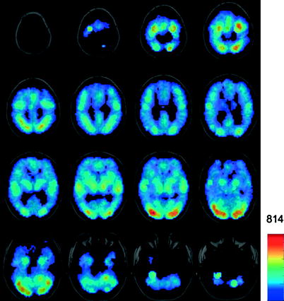
Fig. 7.10
Spatial distribution of “activations” yielded by over 3,000 functional-imaging experiments included in the BrainMap database. The colour scale indicates the number of “activations” at a given location. From Toro et al. (2008b)
Fig. 7.11
Distribution of the different cognitive domains represented by the experiments after the BrainMap classification (a). Histogram of the number of “activated” locations per experiment (b). On average, experiments reported eight locations; a decreasing number of experiments reported large numbers of locations. From Toro et al. (2008b)
The second issue is that of repeatability. As explained in the Preface, population neuroscience is interested in uncovering factors that shape the brain, both from within (genes) and without (social and physical environment). This puts one key requirement on the phenotype: the presence of high test–retest reliability when measured across time (days, weeks) in the same individual. In other words, we need a phenotype that is repeatable (stable over a period of time) so that we can identify with some confidence the genes and/or long-acting environmental/experiential factors that shaped it.
Let us now examine the repeatability of fMRI, as measured in the same individual.18 As reviewed thoroughly by Caceres et al. (2009), we can assess repeatability of fMRI measurements by calculating intraclass correlation coefficients (ICCs).19 This is done by comparing differences in between-subject and within-subject (e.g. across two sessions) variability, relative to the total variation in the sample (the sum of within- and between-subject variability). In fMRI studies, there are several ways one can calculate ICCs for the BOLD response20: (1) for all voxels across the entire brain; (2) for a subset of voxels, constituting a given ROI; and (3) for the mean (or median) BOLD response in a given ROI (Caceres et al. 2009). Evaluating the median of the ICCs (medICCs) calculated for all voxels constituting a given ROI may be particularly useful (Caceres et al. 2009). Using fMRI data collected with two different paradigms in 10 participants across two sessions (three months apart), Caceres et al. (2009) showed that medICCs were ~0.5 for both tasks in the “activated” ROIs; medICCs correlated strongly with the t threshold in the “activated” ROIs and were centred around zero in the WM (Fig. 7.12). It is also important to note that the medICCs varied widely across different ROIs (Fig. 7.13) and, in this sample of 10 participants, their 95 % confidence intervals were quite wide.
Fig. 7.12


Intraclass correlation coefficients (ICCs) calculated from fMRI data obtained in 10 individuals tested on two occasions (3 months apart), using two different paradigms: an auditory task (left panel) and an N-back task (right panel). In the bottom row, the median of the “network” distribution is plotted against the threshold that defines the region. A strong correlation is shown for both tasks. The distribution, corresponding to the white matter with negligible median, is also shown for both tasks. From Caceres et al. (2009)
Related posts:


Stay updated, free articles. Join our Telegram channel
Full access? Get Clinical Tree
