Understanding Research Methods and Statistics: A Primer for Clinicians

George A. Morgan

Jeffrey A. Gliner

Robert J. Harmon

Introduction

Purposes of Research

Research has two general purposes: a) increasing knowledge within the discipline and b) increasing knowledge as a professional consumer of research in order to understand and evaluate research developments within the discipline. For many clinicians, the ability to understand research in one’s discipline may be even more important than making research contributions. Dissemination occurs through an exceptionally large number of professional journals, workshops, and continuing education courses, as well as popular literature. Today’s professional cannot simply rely on the statements of a workshop instructor to determine what should be included in an intervention. Even journal articles need to be scrutinized for weak designs, inappropriate data analyses, or incorrect interpretation of these analyses. Current professionals must have the research and reasoning skills to be able to make sound decisions and support them.

Research Dimensions and Dichotomies

Self-Report versus Researcher Observation

In some studies the participants report to the researcher about their attitudes, intentions, or behavior. In other studies the researcher directly observes and records the behavior of the participant. Sometimes instruments such as heart rate monitors are used by researchers to “observe” the participants’ physiological functioning. Self-reports may be influenced by biases such as the halo effect, or participants may have forgotten or not thought about the topic. Many researchers prefer observed behavioral data. However, sensitive, well trained interviewers may be able to alleviate some of the biases inherent in self-reports.

Quantitative versus Qualitative Research

We believe that this topic is more appropriately thought of as two related dimensions. The first dimension deals with philosophical or paradigm differences between the quantitative (positivist) approach and the qualitative (constructivist) approach to research (1). The second dimension, which is often what people mean when referring to this dichotomy, deals with the type of data, data collection, and data analysis. We think that, in distinguishing between qualitative and quantitative research, the first dimension is the most important.

Positivist Versus Constructivist Paradigms

Although there is disagreement about the appropriateness of these labels, they help us separate the philosophical or paradigm distinction from the data collection and analysis issues. A study could be theoretically positivistic, but the data could be subjective or qualitative. In fact, this combination is quite common. However, qualitative data, methods, and analyses often go with the constructivist paradigm, and quantitative data, methods, and analyses are usually used with the positivist paradigm. This chapter is within the framework of the positivist paradigm, but the constructivist paradigm provides us with useful reminders that human participants are complex and different from other animals and inanimate objects.

Quantitative Versus Qualitative Data, Data Collection, and Analysis

Quantitative data are said to be “objective,” which
indicates that the behaviors are easily and reliably classified or quantified by the researcher. Qualitative data are more difficult to describe. They are said to be “subjective,” which indicates that they are hard to classify or score. Some examples are perceptions of pain and attitudes toward therapy. Usually these data are gathered from interviews, observations, or documents. Quantitative/positivist researchers also gather these types of data but usually translate such perceptions and attitudes into numbers. Qualitative/constructivist researchers, on the other hand, usually do not try to quantify such perceptions; instead, they categorize them.

Data analysis for quantitative researchers usually involves well defined statistical methods, most often providing a test of the null hypothesis. Qualitative researchers are more interested in examining their data for similarities or themes which might occur among all of the participants on a particular topic.

Variables and Their Measurement

Research Problems and Variables

Research Problems

The research process begins with a problem. A research problem is an interrogative sentence about the relationship between two or more variables. Prior to the problem statement, the scientist usually perceives an obstacle to understanding.

Variables

A variable must be able to vary or have different values. For example, gender is a variable because it has two values, female or male. Age is a variable that has a large number of potential values. Type of treatment/intervention is a variable if there is more than one treatment or a treatment and a control group. However, if one studies only girls or only 12-month-olds, gender and age are not variables; they are constants. Thus, we can define variable as a characteristic of the participants or situation that has different values in the study.

Operational Definitions of Variables

An operational definition describes or defines a variable in terms of the operations used to produce it or techniques used to measure it. Demographic variables like age or ethnic group are usually measured by checking official records or simply by asking the participant to choose the appropriate category from among those listed. Treatments are described in some detail. Likewise, abstract concepts like mastery motivation need to be defined operationally by spelling out how they were measured.

Independent Variables

We do not restrict the term independent variable to interventions or treatments. We define an independent variable broadly to include any predictors, antecedents, or presumed causes or influences under investigation in the study.

Active Independent Variables

An active independent variable such as an intervention or treatment is given to a group of participants (experimental) but not to another (control group), within a specified period of time during the study. Thus, a pretest and posttest should be possible.

Attribute Independent Variables

A variable that could not be manipulated is called an attribute independent variable because it is an attribute of the person (e.g., gender, age, and ethnic group) or the person’s usual environment (e.g., child abuse). For ethical and practical reasons, many aspects of the environment (child abuse) cannot be manipulated or given and are thus attribute variables. This distinction between active and attribute independent variables is important for determining what can be said about cause and effect. Research where an apparent intervention is studied after the fact is sometimes called ex post facto. We consider the independent variables in such studies to be attributes.

Dependent Variables

The dependent variable is the outcome or criterion. It is assumed to measure or assess the effect of the independent variable. Dependent variables are scores from a test, ratings on questionnaires, or readings from instruments (electrocardiogram). It is common for a study to have several dependent variables (performance and satisfaction).

Extraneous Variables

These are variables that are not of interest in a particular study but could influence the dependent variable and need to be controlled. Environmental factors, other attributes of the participants, and characteristics of the investigator are possible extraneous variables.

Levels of a Variable

The word level is commonly used to describe the values of an independent variable. This does not necessarily imply that the values are ordered. If an investigator was interested in comparing two different treatments and a no-treatment control group, the study has one independent variable, treatment type, with three levels, the two treatment conditions and the control condition.

We have tried to be consistent and clear about the terms we use; unfortunately, there is not one agreed-upon term for many research and statistical concepts. At the end of most sections, we have included a table similar to Table 2.1.1.1 that lists a number of key terms used in this chapter alongside other terms for essentially the same concept used by some other researchers. In addition to these tables of different terms for the same concept, we have appended a list of partially similar terms or phrases (such as independent variable vs. independent samples) which do not have the same meaning and should be differentiated.

TABLE 2.1.1.1 SIMILAR RELATED TERMS ABOUT VARIABLES

Active independent variable ≈ manipulated variable ≈ intervention ≈ treatment
Attribute independent variable ≈ measured variable ≈ individual difference variable
Dependent variable (DV) ≈ outcome ≈ criterion
Independent variable (IV) ≈ antecedent ≈ predictor ≈ presumed cause ≈ factor
Levels (of a variable) ≈ categories ≈ values ≈ groups ≈ samples

Note. The term we use most often is listed on the left. Similar terms (indicated by ≈) used by other researchers and/or us are listed to the right.

Measurement and Descriptive Statistics

Measurement

Measurement is introduced when variables are translated into labels (categories) or numbers. For statistical purposes, we
and many statisticians (2) do not find the traditional scales of measurement (nominal, ordinal, interval, or ratio) useful. We prefer the following: a) dichotomous or binary (a variable having only two values or levels), b) nominal (a categorical variable with three or more values that are not ordered), c) ordinal (a variable with three or more values that are ordered, but not normally distributed), and d) normally distributed (an ordered variable with a distribution that is approximately normal [bell-shaped] in the population sampled). This measurement classification is similar to one proposed by Helena Chmura Kraemer (personal communication, March 16, 1999).

Descriptive Statistics and Plots

Researchers use descriptive statistics to summarize the data from their samples in terms of frequency, central tendency, and variability. Inferential statistics, on the other hand, are used to make inferences from the sample to the population.

Central Tendency

The three main measures of the center of a distribution are mean, median, and mode (the most frequent score). The mean or arithmetic average takes into account all of the available information in computing the central tendency of a frequency distribution; thus, it is the statistic of choice if the data are normally distributed. The median or middle score is the appropriate measure of central tendency for ordinal-level data.

Variability

Measures of variability tell us about the spread of the scores. If all of the scores in a distribution are the same, there is no variability. If they are all different and widely spaced apart, the variability is high. The standard deviation is the most common measure of variability, but it is appropriate only when one has normally distributed data. For nominal/categorical data, the measure of spread is the number of possible response categories.

Normal Curve

The normal curve is important because many of the variables that we examine in research are distributed in the form of the normal curve. Examples of variables that in the population fit a normal curve are height, weight, IQ, and many personality measures. For each of these examples, most participants would fall toward the middle of the curve, with fewer people at each extreme.

As shown in Figure 2.1.1.1, if a variable is normally distributed, about 68% of the participants lie within one standard deviation from either side of the mean, and 95% are within two standard deviations from the mean. For example, assume that 100 is the average IQ and the standard deviation is 15. The probability that a person will have an IQ between 85 and 115 is .68. Furthermore, only 5% (.05) would be expected to have an IQ less than 70 or more than 130. It is important to be able to conceptualize area under the normal curve in the form of probabilities because statistical convention sets acceptable probability levels for rejecting the null hypothesis at .05 or .01.

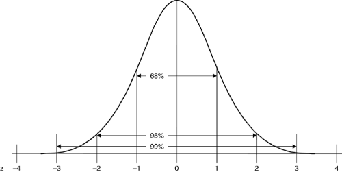FIGURE 2.1.1.1. Frequency distribution and areas under the normal and standardized curve.

Conclusions about Measurement and the Use of Statistics

Table 2.1.1.2 summarizes information about the appropriate use of various kinds of plots and descriptive statistics, given nominal, dichotomous, ordinal, or normal data. Statistics based on means and standard deviation are valid for normally distributed (normal) data. Typically, these data are used in the most powerful (analysis of variance) statistical tests, called parametric statistics. However, if the data are ordered but grossly nonnormal (ordinal), means and standard deviations may not give meaningful answers. Then the median and a nonparametric test based on rank order would be preferred. Nonparametric tests have less power than parametric tests (they are less able to reject the null hypothesis when it should be rejected), but the sacrifice in power for nonparametric tests based on ranks usually is relatively minor. If the data are nominal (unordered), one would have to use the mode or frequency counts. In this case, there would be a major sacrifice in power. It would be misleading to use tests that assume the dependent variable is ordinal or normally distributed when the dependent variable is, in fact, nominal/not ordered. Table 2.1.1.3 provides examples of potentially confusing, essentially equivalent terms about measurement and descriptive statistics.

Measurement Reliability

Measurement reliability and measurement validity are two parts of overall research validity, the quality of the whole study. Reliability refers to consistency of scores on a particular instrument. It is incorrect to state that a test is reliable because reliability takes into account the sample that took the test. For example, there may be strong evidence for reliability for adults, but scores of depressed adolescents on this test
may be highly inconsistent. When researchers use tests or other instruments to measure outcomes, they need to make sure that the tests provide consistent data. If the outcome measure is not reliable, then one cannot accurately assess the results.

TABLE 2.1.1.2 SELECTION OF APPROPRIATE DESCRIPTIVE STATISTICS AND PLOTS

	Nominal	Dichotomous	Ordinal	Normal
Graphic Depiction (Plot)
Frequency Distribution	Yes^a	Yes	Yes	OK^b
Bar chart	Yes	Yes	Yes	OK
Histogram	No^c	No	OK	Yes
Frequency polygon	No	No	OK	Yes
Box and whiskers plot	No	No	Yes	Yes
Central Tendency
Mean	No	OK	Of ranks, OK	Yes
Median	No	OK = mode	Yes	OK
Mode	Yes	Yes	OK	OK
Variability
Range	No	Always 1	Yes	Yes
Standard deviation	No	No	Of ranks, OK	Yes
Interquartile range	No	No	OK	OK
How many categories	Yes	Always 2	OK	Not if truly continuous
Shape
Skewness	No	No	Yes	Yes
^aYes means a good choice with this level of measurement. ^bOK means OK to use, but not the best choice at this level of measurement. ^cNo means not appropriate at this level of measurement.

Conceptually, reliability is consistency. When evaluating instruments it is important to be able to express reliability numerically. The correlation coefficient, often used to evaluate reliability, is usually expressed as the letter r, which indicates the strength of a relationship. The values of r range between -1 and +1. A value of 0 indicates no relationship between two variables or scores, whereas values close to -1 or +1 indicate very strong relationships between two variables. A strong positive relationship indicates that people who score high on one test also score high on a second test. To say that a measurement is reliable, one would expect a coefficient between +.7 and +1.0. Others have suggested even stricter criteria. For example, reliability coefficients of .8 are acceptable for research, but .9 is necessary for measures that will be used to make clinical decisions about individuals. However, it is common to see published journal articles in which one or a few reliability coefficients are below .7, usually .6 or greater. Although correlations of -.7 to -1.0 indicate a strong (negative) correlation, they are totally unacceptable as evidence for reliability.

TABLE 2.1.1.3 SIMILAR TERMS ABOUT MEASUREMENT

Categorical variable ≈ usually nominal, but variables may have discrete ordered categories
Dichotomous ≈ binary ≈ dummy variable ≈ nominal with two categories
Interval scale ≈ numeric ≈ continuous variable ≈ quantitative ≈ scale data
Mean ≈ average ≈ arithmetic average
Median ≈ midpoint
Normal ≈ (approximately) normally distributed variable ≈ interval and ratio data ≈ quantitative ≈ continuous
Nominal scale ≈ unordered categorical variable ≈ qualitative ≈ discrete
Ordered variable ≈ ordinal or interval scale
Ordinal scale ≈ unequal-interval scale ≈ discrete ordered categorical variable
Range ≈ spread

Note. The term we use most often is listed on the left. Similar terms (indicated by ≈) used by other researchers and/or us are listed to the right.

There are four different types of evidence for reliability, such as test-retest reliability, that are listed in Table 2.1.1.4, along with synonyms that you may see in the literature. In addition, there are many different methods to compute these different types of reliability. See Morgan, Gliner and Harmon (3) for specifics about these approaches to assessing reliability.

TABLE 2.1.1.4. SIMILAR TERMS ABOUT MEASUREMENT RELIABILITY

Alternate forms reliability ≈ equivalent forms ≈ parallel forms ≈ coefficient of equivalence
Internal consistency reliability ≈ interitem reliability ≈ Cronbach’s alpha
Interrater reliability ≈ interobserver reliability
Measurement reliability ≈ reliability ≈ test, instrument, or score reliability
Test-retest reliability ≈ coefficient of stability

Note. The term we use most often is listed on the left. Similar terms (indicated by ≈) used by other researchers and/or us are listed to the right.

Measurement Validity

Validity is concerned with establishing evidence for the use of a particular measure or instrument in a particular setting with a particular population for a specific purpose. Here we will discuss what we call measurement validity; others might use terms such as test validity, score validity, or just validity. We use the modifier measurement to distinguish it from internal, external, and overall research validity and to point out that it is the measures or scores that provide evidence for validity. It is inappropriate to say that a test is “valid” or “invalid.” Note also that an instrument may produce consistent data (provide evidence for reliability), but the data may not be a valid index of the intended construct.

In research articles, there is usually more evidence for the reliability of the instrument than for the validity of the instrument because evidence for validity is more difficult to obtain. To establish validity, one ideally needs a “gold standard” or “criterion” related to the particular purpose of the measure. To obtain such a criterion is often not an easy matter, so other types of evidence to support the validity of a measure are necessary.

There are five broad types of evidence to support the validity of a test or measure: a) content, b) responses, c) internal structure, d) relations to other variables, and e) the consequences of testing (4). Note that the five types of evidence are not separate types of validity and that any one type of evidence is insufficient. Validation should integrate all the pertinent evidence from as many of the five types of evidence as possible. Preferably validation should include some evidence in addition to content evidence, which is probably the most common and easiest to obtain. Table 2.1.1.5 shows the traditional names for the types of validity evidence and how they line up with the types of evidence from the current standards (4).

Evaluation of evidence for validity is often based on correlations with other variables, but there are no well established guidelines. Our suggestion is to use Cohen’s (5) guidelines for interpreting effect sizes, which are measures of the strength of a relationship. We describe several measures of effect size and how to interpret them. Cohen suggested that generally, in the applied behavioral sciences, a correlation of r = .5 could be considered a large effect, and in this context we would consider r = .5 or greater to be strong support for measurement validity. In general, an acceptable level of support would be provided by r ≥ .3, and some weak support might result from r ≥ .1, assuming that such an r was statistically significant. However, for concurrent, criterion evidence, if the criterion and test being validated are two similar measures of the same concept (e.g., IQ), the correlation would be expected to be very high, perhaps .8 or .9. On the other hand, for convergent evidence, the measures should not be that highly correlated because they should be measures of different concepts. If the measures were very highly related, one might ask whether they were instead really measuring the same concept.

TABLE 2.1.1.5. SIMILAR TERMS ABOUT VALIDITY

Concurrent validity ≈ now part of “evidence based on relations to other variables”
Construct validity ≈ now part of “evidence based on relations to other variables”
Content validity ≈ now part of “content evidence for validity”
Convergent validity ≈ now part of “evidence based on relations to other variables”
Criterion validity ≈ now part of “evidence based on relations to other variables”
Discriminant validity ≈ now part of “evidence based on relations to other variables”
Face validity ≈ (no longer used)
Factorial validity ≈ now part of “evidence based on internal structure”
Predictive validity ≈ now part of “evidence based on relations to other variables”
Validity (of a specific measure) ≈ measurement validity ≈ test, instrument, or score validity
Validity (of the design of a study) ≈ research validity ≈ internal or external validity

Note. In this table the traditional term is provided on the left. Similar terms, used in the current standards (4) are on the right. (See also Figure 2.1.1.7.)

The strength of the evidence for the measurement of validity is extremely important for research in applied settings because without measures that have strong evidence for validity the results of the study can be misleading. Validation is an ongoing, never fully achieved, process based on integration of all the evidence from as many sources as possible.

Research Approaches, Questions, and Designs

Quantitative Research Approaches

Our conceptual framework includes five quantitative research approaches (randomized experimental, quasiexperimental, comparative, associational, and descriptive). This framework is helpful because it provides appropriate guidance about inferring cause and effect.

Figure 2.1.1.2 indicates that the general purpose of four of the five approaches is to explore relationships between or among variables. This is consistent with the notion that all common parametric statistics are relational and with the typical phrasing of research questions and hypotheses as investigating the relationship between two or more variables. Figure 2.1.1.2 also indicates the specific purpose, type of research question, and general type of statistic used in each of the five approaches.

Research Approaches with an Active Independent Variable

Randomized Experimental Research Approach

This approach provides the best evidence about cause and effect. For a research approach to be called randomized experimental, two criteria must be met. First, the independent variable must be active (be a variable that is given to the participant, such as a treatment). Second, the researcher must randomly assign participants to groups or conditions prior to the intervention; this is what differentiates experiments from quasiexperiments. More discussion of specific quasiexperimental and randomized designs is provided below.

Quasiexperimental Research Approach

Researchers do not agree on the definition of a quasiexperiment. Our definition is that there must be an active/manipulated independent variable, but the participants are not randomly assigned to the groups. In much applied research participants are already in groups such as clinics, and it is not possible to change those assignments and divide the participants randomly into experimental and control groups.

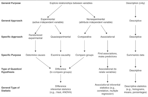FIGURE 2.1.1.2. Schematic diagram showing how the general type of statistic and hypothesis or question used in a study corresponds to the purposes and the approach.

Research Approaches That Have Attribute Independent Variables

In most ways the associational and comparative approaches are similar. We call both nonexperimental approaches, as shown in Figure 2.1.1.2. The distinction between them, which is implied but not stated in most research textbooks, is in terms of the number of levels of the independent variable.

It is common for survey research to include both comparative and associational as well as descriptive research questions, and therefore to use all three approaches. It is also common for experimental studies to include attribute independent variables, such as gender, as well as an active independent variable and thus to use both experimental and comparative approaches. The approaches are tied to types of independent variables and research questions, not necessarily to whole studies.

Comparative Research Approach

Like randomized experiments and quasiexperiments, the comparative approach, which is sometimes called causal-comparative, or ex post facto, usually has a few levels (typically two to four) or categories for the independent variable and makes comparisons between groups.

Associational Research Approach

This approach is similar to the comparative approach because the independent variable is an attribute. In this approach, the independent variable is often continuous or has a number of ordered categories, usually five or more. We prefer to label this approach associational rather correlational, used by some researchers, because the approach is more than, and should not be confused with, a specific statistic.

Descriptive Research Approach

The term descriptive research refers to questions and studies that use only descriptive statistics, such as averages, percentages, histograms, and frequency distributions, which are not tested for statistical significance. This approach is different from the other four in that only one variable is considered at a time so that no comparisons or associations are determined. Although most research studies include some descriptive questions (at least to describe the sample), few stop there.

Research Questions and Hypotheses

Three Types of Basic Hypotheses or Research Questions

A hypothesis is a predictive statement about the relationship between two or more variables. Research questions are similar to hypotheses, but they are in question format. Research questions can be further divided into three types: difference questions, associational questions, and descriptive questions (see Figure 2.1.1.2).

For difference questions, one compares groups or levels derived from the independent variable in terms of their scores on the dependent variable. This type of question typically is used with the randomized experimental, quasiexperimental, and comparative approaches. For an associational question, one associates or relates the independent and dependent variables. Our descriptive questions are not answered with inferential statistics; they merely describe or summarize data.

As implied by Figure 2.1.1.2, it is appropriate to phrase any difference or associational research question as simply a relationship between the independent variable(s) and the dependent variable. However, we think that phrasing the research questions/hypotheses as a difference between groups or as a relationship between variables helps match the question
to the appropriate statistical analysis. Table 2.1.1.6 shows the terms other researchers sometimes use that correspond to those for our research approaches and questions.

TABLE 2.1.1.6 SIMILAR TERMS ABOUT RESEARCH APPROACHES AND QUESTIONS

Associational approach ≈ correlational ≈ survey ≈ descriptive
Associational questions ≈ correlational questions
Comparative approach ≈ causal-comparative ≈ ex post facto
Descriptive approach ≈ exploratory research
Difference questions ≈ group comparisons
Nonexperimental research (comparative, associational, and descriptive approaches) ≈ some writers call all three descriptive

Note. The term we use most often is listed on the left. Similar terms (indicated by ≈) used by other researchers and/or us are listed to the right.

Experimental Designs

We describe here specific designs for both quasiexperiments and randomized experiments. This should help the reader visualize the independent variables, levels of these variables, and whether the participants are assessed on the dependent variable more than once.

Quasiexperimental Designs

The randomized experimental and quasiexperimental approaches have an active independent variable, which has two or more values, called levels. The dependent variable is the outcome measure or criterion of the study.

In both randomized and quasiexperimental approaches, the active independent variable has at least one level that is some type of intervention given to participants in the experimental group during the study. Usually there is also a comparison or control group, which is the other level of the independent variable. There can be more than two levels or groups (e.g., two or more different interventions plus one or more comparison groups).

The key difference between quasiexperiments and randomized experiments is whether the participants are assigned randomly to the groups or levels of the independent variable. In quasiexperiments random assignment of the participants is not done; thus, the groups are always considered to be nonequivalent, and there are alternative interpretations of the results that make definitive conclusions about cause and effect difficult. For example, if some children diagnosed with attention-deficit/hyperactivity disorder were treated with stimulants and others were not, later differences between the groups could be due to many factors. Families who volunteer (or agree) to have their children medicated may be different, in important ways, from those who do not. Or perhaps the more disruptive children were given stimulants. Thus, later problem behaviors (or positive outcomes) could be due to initial differences between the groups.

Poor Quasiexperimental Designs

Results from these designs (sometimes called preexperimental) are hard to interpret and should not be used. These designs lack a comparison (control) group, a pretest, or both.

Better Quasiexperimental Designs

Pretest-Posttest Nonequivalent-Groups Design

As with all quasiexperiments, there is no random assignment of the participants to the groups in this design. First, measurements (O₁) are taken on the groups prior to an intervention. Then one group (E) receives a new treatment (X), which the other (comparison) group (C) does not receive (∼X); often the comparison group receives the usual or traditional treatment. At the end of the intervention period, both groups are measured again (O₂) to determine whether there are differences between the two groups. The design is considered to be nonequivalent because the participants are not randomly assigned (NR) to one or the other group. Even if the two groups have the same mean score on the pretest, there may be characteristics that have not been measured that may interact with the treatment to cause differences between the two groups that are not due strictly to the intervention. The following diagram illustrates the procedures for the pretest-posttest nonequivalent groups design:

NR	E	O₁	X	O₂
NR	C	O₁	∼X	O₂

Table 2.1.1.7 summarizes two issues that determine the strength (from weak to strong) of the pretest-posttest nonequivalent groups design. These designs vary, as shown, on whether the treatments are randomly assigned to the groups or not and on the likelihood that the groups are similar in terms of attributes or characteristics of the participants. In none of the quasiexperimental designs are the individual participants randomly assigned to the groups, so the groups are always considered nonequivalent, but the participant characteristics may be similar if there was no bias in how the participants were assigned (got into) the groups.

Time-Series Designs

Time-series designs are different from the more traditional designs discussed above because they have multiple measurement (time) periods rather than just the pre- and post-periods. These designs often are referred to as interrupted time series because the treatment interrupts the baseline from posttreatment measures. The two most common types are single-group time-series designs and multiple-group time-series designs (6). Within each type, the treatment can be temporary or continuous. The logic behind any time-series
design involves convincing others that a baseline (several pretests) is stable prior to an intervention so that one can conclude that the change in the dependent variable is due to the intervention and not other environmental events or maturation. It is common in time-series designs to have multiple measures before and after the intervention, but there must be multiple (at least three) pretests to establish a baseline. One of the hallmarks of time-series designs is the visual display of the data, which are often quite convincing. However, these visual displays also can be misleading due to the lack of independence of the data points, and therefore always must be statistically analyzed.

TABLE 2.1.1.7. ISSUES THAT DETERMINE THE STRENGTH OF QUASIEXPERIMENTAL DESIGNS

Strength of Design	Random Assignment of Treatments to Intact Groups	Participant Characteristics Likely to Be Similar
Poor (or pre)	No	No, because no comparison group or no pretest
Weak	No	Not likely, because participants decide which group to join (self-assign to groups)
Moderate	No	Maybe, because participants did not self-assign to groups and no known assignment bias
Strong	Yes	Maybe, because participants did not self-assign to groups and no known assignment bias