Fig. 8.1
Representative cortical myelination in the marmoset. A 40 μm–thick coronal histological section stained for myelin using a modified Gallyas silver staining method. At the whole mount level of magnification showing half of the brain, distinct dense areas of staining are seen that correspond to specific cortical areas (for example, the primary auditory cortex [A1]). At 2.5 times magnification, dark-stained fibers can be seen running vertically from the white matter through Layers VI and V. At 20 times magnification in Layer IV, the fibers are arborized, and vertical and horizontal stained branches can be seen. There is little myelin staining through Layers III-I (WM, white matter. The asterix denotes the same blood vessel in each magnification.) (From Bock et al. 2011)
8.4 MRI of Myelination
MRI is sensitive to a number of different physical properties of tissue, including the longitudinal relaxation time of protons (T1), the transverse relaxation time of protons (T2), the magnitude and direction of water diffusion in the tissue, and the magnetic susceptibility of the tissue (detected as T2* contrast). In the brain, the presence of myelin in white matter structures causes a large difference in the MR properties of the tissue in these structures relative to the properties in gray matter structures. These differences give rise to the exquisite contrast seen on anatomical MRIs that highlights gross brain anatomy. Imaging cortical myelin is based on the same MR contrast mechanism by which myelin in white matter tracts produces contrast between major gray and white matter structures of the central nervous system (CNS). In fact, it has been shown that the Stripe of Gennari, a heavily myelinated structure in V1, can be identified in humans on T1-weighted (Barbier et al. 2002), T2-weighted (Carmichael et al. 2006; Trampel et al. 2011), and T2 *-weighted images (Fukunaga et al. 2010).
In marmosets, we have measured the difference in T1 between regions of the cortex with a low myelin content and a high myelin content to be 270 ms at 7 T (Bock et al. 2009). Although this difference is smaller than the difference in T1 between gray matter with a low myelin content and white matter of 610 ms, it is sufficient to generate intracortical contrast on an MRI. We image myeloarchitecture based on this T1-weighted contrast using a three dimensional (3D) T1-weighted MRI sequence commonly used to image gross neuroanatomy that we have optimized to increase the contrast for imaging differences in cortical myelination (Bock et al. 2009). We choose to image based on T1 contrast because T1-weighted sequences are highly amenable for 3D high resolution anatomical neuroimaging.
To visualize myeloarchitecture across the entire cortex, we image isoflurane-anaesthetized marmosets for roughly 4 h with our 3D sequence to produce an MRI of the whole brain at 150 μm isotropic resolution. In Fig. 8.2, we show 2D coronal slices from a representative 3D MRI of a marmoset and corresponding matched histological sections stained for myelin. There is a very good spatial correspondence between known highly myelinated regions of the marmoset cortex and signal enhancement in the MRI. This importantly suggests that MRI is sensitive to myelin in the cortex, although there is a remote possibility that we are visualizing another feature of the cortex that is highly co-localized with myelin (such as non-heme iron (Fukunaga et al. 2010)), which would also brighten a T1-weighted MRI.
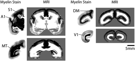
Fig. 8.2
40 μm thick coronal myelin-stained histology sections through the marmoset brain and corresponding 167 μm slices from an in vivo T1-weighted MRI. The MRIs are masked to only show the brain and presented on a gray background to make the edges of the cortex visible. The number in the upper right hand corner of each MRI indicates the order of the slices from rostral to caudal. (A1, primary auditory cortex; S1, primary somatosensory cortex; MT, middle temporal area; DM, dorsomedial area; V1, primary visual cortex). Note that the contrast is reversed in the two types of images, with myelinated areas appearing dark in the histological sections and bright in the MRI (Adapted from Bock et al. 2009)
8.5 Visualization of MRI Data
While it is possible to explore myeloarchitecture in marmosets in 2D slices extracted from a 3D MRI, the patterns can be best appreciated if viewed across the cortical surface. This requires the MRI data to be surface rendered, which proceeds as follows (Fig. 8.3).
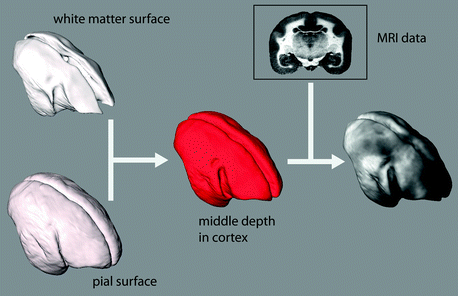
Fig. 8.3
Surface processing of 3D MRI data. The white matter surface and the pial surface are first obtained from the 3D MRI data using semi-automatic image segmentation. The middle distance between these surfaces is then computed to produce a new surface at a middle depth in the cortex. The MRI intensity data at this middle depth is then projected on the surface to form a map
First, the inner and outer surfaces of the cortex must be segmented (Tosun et al. 2004). In our marmoset images, we segment the boundary between the cortex and the underlying white matter based on intensity thresholding. This is robust because there is such high contrast between gray and white matter in our images. The pial boundary is more difficult to segment because there is less contrast in the images between cortical tissue and the cerebral spinal fluid (CSF) or dura matter. We begin with a rough atlas-based segmentation of this boundary, followed by a manual correction. Once the pial and white matter boundaries of the cortex are segmented we create a surface mesh of each, then calculate normals between these surfaces. Next, we compute a new surface at a distance between the pial and white matter surfaces along these normals which then lies at a middle depth in the myelinated layers of the cortex. For instance, this middle surface lies in the Stripe of Gennari in V1 and in Layer IV in S1. For display purposes, the MRI intensity data at the middle surface depth is displayed on the surface. To aid visualization, we display the grayscale MRI intensity data using an orange colourmap in our whole-cortex maps (Fig. 8.4). The brighter regions in the map represent regions of the marmoset cortex with a high myelin content. The surface-rendered map can be viewed from different angles (Fig. 8.5) to reveal myeloarchitecture over the entire cortex. This is perhaps the best way to appreciate the patterns of myeloarchitecture in the marmoset free of distortion, although a surface map can also be digitally flattened (Fig. 8.6) to show all heavily myelinated regions in a single view, which is similar to what one would see with flatmounting on histology.
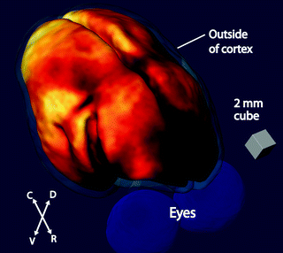
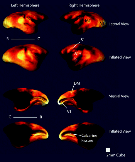
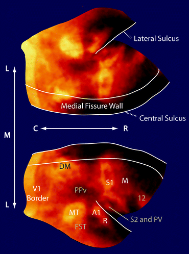
Fig. 8.4
3D map of myeloarchitecture in a representative 3-year-old male common marmoset. The figure shows a view of a 3D map of the cortex in a marmoset centered on the dorsal parietal cortex. Here, the MRI intensity data are displayed using an orange colormap to highlight contrast and areas of enhancement represent cortical areas with high myelin content. The map is placed at a middle depth in the cortex, and the surface corresponding to the outside of the cortex is shown in light transparent blue. (C, caudal; R, rostral; V, ventral; D, dorsal.)
Fig. 8.5
Multiple views of the surface-rendered cortex from Fig. 8.4. Each view is paired with an inflated view of the cortex to show myeloarchitecture the cortical folds of the lateral sulcus and calcarine fissure. (C, caudal; R, rostral) (Several major myelinated cortical regions are labeled: V1, primary visual area; MT, middle temporal area; A1, primary auditory area; R, rostral auditory area; S1, primary somatosensory cortex; DM, dorsomedial area)
Fig. 8.6
Flattened map of myeloarchitecture in a representative 3-year old female common marmoset. The dorsal cortical surface from a 3D map is flattened with the major enhancing areas labeled. Note that the flattening produces spatial distortions in the surface; however, the flattening allows for easier visualization of cortical features and their spatial relationships. (C, caudal; R, rostral; L, lateral; M, medial) (Major myelinated cortical regions are labeled in white: V1, primary visual area; MT, middle temporal area; A1, primary auditory area; R, rostral auditory area; S1, primary somatosensory cortex; M, motor cortex including primary and premotor areas and the frontal eye fields) (Cortical features are labeled in gray: DM, dorsomedial area; PPv, ventral posterior parietal cortex; FST, fundus of the superior temporal area; S2, secondary somatosensory cortex; PV, parietal ventral area; 12, area 12) (Adapted from Bock et al. 2011)
8.6 Overall Myeloarchitecture in the Marmoset
Overall, we observe in our maps of myeloarchitecture five highly-myelinated major cortical regions in the marmoset: the primary sensory regions A1, S1, and V1, and regions in the extrastriate visual pathway: the middle temporal region (MT) and the dorsomedial region (DM). It makes sense that the primary sensory regions would be highly myelinated so as to improve the speed of input signals. The axons traversing visual associated areas too are likely myelinated to also speed visual responses in the brain. The location and geometry of major myelinated regions agree well with previous studies of myeloarchitecture in the marmoset brain. Interestingly, we do not see strong enhancement in the primary motor cortex (M1) in the marmoset, although this region is one of the most heavily myelinated in humans (Hopf 1956). This highlights potential differences in neuroanatomy in small, New World primates versus large Old World primates. Aside from strong enhancements in major cortical regions, there are also fainter enhancements in regions that can be identified because they are surrounded by cortex with a very low myelin content (e.g. area 12 in the frontal cortex) or are specifically identified by their low myelin content (e.g. the ventral posterior parietal cortex, PPv (Rosa et al. 2009)). Specific features of marmoset myeloarchitecture observable with MRI are discussed in further detail below.
8.7 Myeloarchitecture of Specific Regions
8.7.1 Auditory Regions
The primary auditory cortex, A1, in marmosets is a prominent myelinated feature of the temporal lobe (Pistorio et al. 2006), which is unsurprising as the marmoset has a well-developed repertoire of tonal vocalizations, a similar hearing range as humans (Aitkin and Park 1993), and can even discriminate the pitch of complex tones (Bendor and Wang 2005). We readily identify A1 in our images in the dorsal temporal cortex, extending into the lateral sulcus. Continuous with A1 is another myelinated auditory area, the rostral auditory area (R). Since there is no discernible border between A1 and R, they are treated as a single region in our maps. In humans, short T1s have also been noted in A1 and related to a high myelin content (Sigalovsky et al. 2006). Interestingly, that study measured lower T1s in Heschl’s gyrus on the left side of the brain than on the right, suggesting that there are asymmetries in cortical myelination that may reflect specialized functional processing. It would be interesting in a future study to see if the same asymmetries are present in marmosets, either in the T1 values, or in the size of A1.
8.7.2 Somatosensory Regions
Another highly myelinated primary sensory area in the marmoset is the primary somatosensory cortex S1 (also referred to as area 3b). This area features a characteristic somatotopic organization, with sub-areas corresponding to representations of different parts of the body within S1 being distinguished by patchy regions of high myelination surrounded by poorly myelinated regions (Krubitzer and Kaas 1990). S1 is strongly enhanced in our T1-weighted images (Figs. 8.2 and 8.3), and the patchiness is also apparent. Within the medial wall of the lateral sulcus the much smaller secondary somatosensory area (Krubitzer and Kaas 1990), S2, can also be seen. This is continuous with another myelinated region, the parietal ventral area (PV) (Krubitzer and Kaas 1990) and since there is no discernible border again, the two regions are treated as one in our maps.
8.7.3 Visual Regions
V1 was one of the first cortical areas to be segregated based on its high myelin content (Gennari 1782). Since, the stripe of Gennari has been the major structural feature used to distinguish V1 from other cortical areas both in monkeys (Pessoa et al. 1992), as well in humans (Clarke and Miklossy 1990). V1 is the area that has been most extensively visualized with MRI in humans in vivo and ex vivo (Clark et al. 1992; Barbier et al. 2002; Walters et al. 2003; Eickhoff et al. 2005; Bridge et al. 2005; Bridge and Clare 2006; Hinds et al. 2008). From a technical standpoint, it is actually one of the most difficult myelinated areas to image because of the high spatial resolution needed to visualize the stripe of Gennari (Peters and Sethares 1996). All the other highly myelinated areas we identified contain myelinated fibers spanning multiple lower layers of the cortex which make them easier to image. In V1, the myelinated fibers are mostly confined to just layer IV, although there is light myelination of the deeper cortical layers too. The border between V1 and the secondary visual cortex (V2) is readily delineated since the density of myelin throughout the layers of V2 is far lower than in V1. The rostral border of V2 is not discernible in our map because there is not a great enough difference in myelination between V2 and adjoining rostral areas. The extent of V2 is traditionally visualized using cytochrome oxidase staining (Jeffs et al. 2009), rather than myelin staining, and our inability to delineate V2 in our map shows the limitation of describing cortical organization based on only one contrast mechanism.
Another visual area that has been extensively studied in monkeys based on myeloarchitecture is the middle temporal area, MT (Van Essen et al. 1981; Bourne et al. 2007), which has been implicated in processing visual motion (Ungerleider and Desimone 1986). In the marmoset, MT is a heavily myelinated region situated dorsal and posterior to the temporal sulcus. Since the myelinated fibers span from layer III to VI (Bourne et al. 2007), we were able to readily identify MT in both our T1 maps and in our T1-weighted images. The corresponding homologous area in humans, V5/MT, has been identified using both anatomical MRI with myelin-based contrast, and with functional MRI using a stimulation protocol selective for moving stimuli (Walters et al. 2003). Ventral and anterior to MT is an enhancing area corresponding to the fundus of the superior temporal area (FST) (Rosa and Elston 1998).
Another major enhancing region we identified in the visual pathway is the dorsomedial area (DM). The shape and extent of DM is not well defined in the literature based on its myelination; however, it has strong enhancement and we have labeled it in our map although its actual borders are indistinct. DM is similar in size to MT and receives projections from V1 (Rosa and Schmid 1995; Lyon and Kaas 2001).
8.7.4 Motor Regions and Frontal Cortex
In the parietal-frontal cortex of our map, the motor areas are visible. Even though these output areas contain less myelin than the primary sensory areas, their caudal border is readily identified because of contrast with S1 which is heavily myelinated and their rostral border is visible as there is very little myelin in the rest of the frontal cortex. Although the large motor area, M, we have identified in our map contains many subdivisions, including the primary motor cortex, the premotor areas, and the frontal eye fields (Burman et al. 2008; Burish et al. 2008), there is little contrast between these regions, so they must be grouped into a common area. Area 12 in the dorsolateral and orbital frontal cortex is relatively well-myelinated (Burman and Rosa 2009) and is easily identified in our map. Interestingly, this area is an important source of projections to the heavily myelinated MT area (Burman et al. 2006).
8.8 Implications
The implications of being able to visualize in vivo myeloarchitecture in marmosets revolve around our new ability to non-invasively and robustly observe cortical organization in these monkeys. While it has been possible to observe patterns of myeloarchitecture in marmosets previously using histology, it required sacrifice of the animal, which precluded longitudinal studies and increased the number of animals required for morphological studies.
We have performed preliminary morphological studies to show our technique can quantitatively summarize cortical organization in the marmoset. We measured the surface areas of the major enhancing areas in maps from four female monkeys: two three-year old young adults, and two eight-year old middle aged monkeys (Abbott et al. 2003) (see Fig. 8.7 and Table 8.1). The low standard deviations in our measurements suggest that the size of cortical areas may be largely preserved over different individuals, although a more statistically rigorous study with a large number of animals would be required to confirm this. This type of study is easily performed now, since no animals need to be sacrificed. Comparing measurements between hemispheres, we again see little variation, although more animals would also be needed to statistically confirm this.
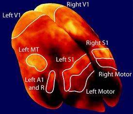
Table 8.1
Surface area measurements


