Computational Anatomy
Jack J. Lin
John C. Mazziotta
Introduction
Improvements in magnetic resonance imaging (MRI) technology have significantly improved signal-to-noise characteristics, allowing in vivo visualization of brain anatomic structures at relatively high (<1 mm) resolution. With the use of mathematical modeling in computational anatomy, these high-resolution images can be manipulated to detect subtle differences in neuroanatomy beyond what is possible qualitatively with the human eye.4
Previously, quantitative magnetic resonance tools have focused on manually delineated volumes to assess brain size and regions of interest such as the hippocampus and the amygdala.9,21 Volumetric changes may not be sensitive in detecting early or subtle changes. Even when volumetric changes are detected, these methods lack regional specificity because they cannot map the exact location of structural abnormalities. Region-of-interest studies can only evaluate the specific brain area in question, without assessing other structurally or functionally connected regions. Finally, volumetric studies cannot provide information relating to the change in shape of the neuroanatomic structure that maybe vulnerable to the underlying epileptic disease process.
With the advances in computational speed and automated image analysis, the emerging field of computational anatomy has recently been employed in epilepsy. Computational anatomy is the effort to develop algorithms that use mathematical techniques such as differential geometry, numerical analysis, and partial differential equations to model anatomic structures in brain image data.46 Some of these techniques can be applied to the entire brain without a priori bias to study global changes associated with epilepsy.10,11,30 Other techniques extend previous region-of-interest volumetric studies to map the precise location of atrophy and shape deviation in selected structures, such as the hippocampus.25,33 These algorithms detect cross-sectional differences between an epilepsy group and appropriately matched controls or prospective changes over time. The regional-specific changes can also be related to clinical variables to elucidate the underlying structure–function relationship. These studies provide a better understanding of the widespread cerebral changes associated with epilepsy, clinical factors that correlate with these anatomic differences, and anatomic predictors of surgical outcome. In this chapter, we review some of the basic algorithms of computational anatomy and discuss specific computational methods that have been employed in epilepsy. Finally, we highlight some of the important clinical findings resulting from these efforts.
Overview of Algorithms
Algorithms in computational anatomy can be divided into methods that evaluate whole brain or cortical structures versus those used to assess subcortical structures. Most whole-brain or cortical algorithms have all or some of the following steps in common: (a) brain extraction (remove voxels containing brain tissue from nonbrain voxels), (b) tissue classification (partition the voxels into gray and white matter and cerebrospinal fluid [CSF]), and (c) spatial normalization or registration. The great variability in human brain anatomy presents a particular challenge in developing strategies to average and compare brain structures across individuals. This is precisely the goal of spatial normalization, a pivotal step that differs greatly in different brain-mapping algorithms. Voxel-based morphometry and cortical pattern matching illustrate two potential approaches to some of these issues.2,50 When studying subcortical structures such as the hippocampus, computational anatomists are no longer satisfied with volumetric information alone. Large-deformation, high-dimensional brain mapping (HDBM-LD) is a method for assessing morphologic shape changes such as inward or outward deviations that may give subtle but important clues to the underlying pathophysiologic process.17,26 Surface-based anatomic mapping is another technique that maps the precise location of the atrophy pattern.33,52 Specific disease processes may preferentially affect more vulnerable anatomic regions, and detailed visualization may further our understanding of the pathology. Diffusion tensor imaging (DTI) with probabilistic tractography allows the assessment of individual white matter bundle structural integrity that is not possible with conventional structural imaging.
Most computational methods require high-spatial-resolu-tion MRI with clear tissue differentiation among gray and white matter and CSF. Typically, T1-weighted, three-dimensional (3D) MRI such as spoiled-gradient-echo (SPGR) or magnetization-prepared rapid gradient-echo sequence (MP-RAGE) acquired on a 1.5- or 3-T magnet and 1-mm isotropic voxels across the entire cranium provides sufficient anatomic resolution for these analysis. These T1-weighted raw images can be improve with MR sequences using centric phase encoding rather than linear phase encoding.18 Radiofre-quency inhomogeneity can be further corrected with a special excitation pulse to compensate these effects.19 More recently, the development of the multichannel head coil array (iPAT-coil) has allowed parallel acquisition of independently reconstructed images, thus reducing scanner time and improving signal-to-noise characteristics.56
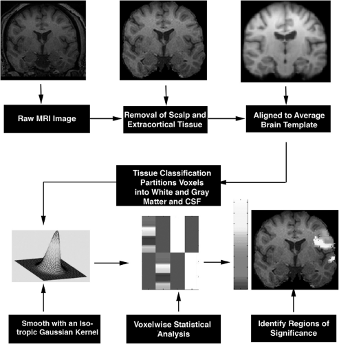 FIGURE 1. Steps in voxel-based morphometry. Scalp and extracortical tissues are removed from raw images, and the resulting brain images are normalized to a standard template. Gray and white matter and cerebrospinal fluid (CSF) are automatically classified based on voxel intensity values. Normalized images are smoothed with an isotropic Gaussian kernel. Voxelwise statistical analysis based on generalized linear model is applied to the images to identify regions of significance. MRI, magnetic resonance imaging. (See the color insert.) |
Because temporal lobe epilepsy is the most common form of epilepsy, studies are particularly interested in defining lateral and mesial temporal lobe structural deficits. However, the temporal lobe, particularly the medial aspect, is partially surrounded by bone and tissue interfaces such as nasal sinuses, ear cavities, and perforated bone and thus is prone to susceptibility artifacts. Magnetic susceptibility differences between tissue/air and bone/tissue interfaces result in magnetic field gradients, which lead to intravoxel phase dispersion and image distortion. These susceptibility artifacts can affect computational results,
and steps have been proposed to compensate for this static field effect. Spiral acquisition sequences use shorter TE and a single-shot acquisition, which can reduce geometric distortion.23 Another approach to reducing local background gradient is to use Z-shimming, in which slice refocusing gradients are collected and combined.22 More recently multiple array parallel image techniques have been employed to reduce susceptibility artifact and increase signal-to-noise characteristics (8).
and steps have been proposed to compensate for this static field effect. Spiral acquisition sequences use shorter TE and a single-shot acquisition, which can reduce geometric distortion.23 Another approach to reducing local background gradient is to use Z-shimming, in which slice refocusing gradients are collected and combined.22 More recently multiple array parallel image techniques have been employed to reduce susceptibility artifact and increase signal-to-noise characteristics (8).
Voxel-Based Morphometry
Voxel-based morphometry (VBM) is a whole-brain analysis tool in which voxelwise statistical comparisons of local gray matter concentrations are made between two groups of subjects.2 VBM algorithms involve spatial normalization, tissue segmentation, smoothing, and finally application of statistical analysis to localize and infer group differences (Fig. 1). Spatial normalization involves the transformation of all of the subjects’ images to the same stereotactic space to remove global brain difference between subjects. This step is important because the goal of VBM analysis is to detect regional brain tissue concentration, and, therefore, it must first remove global differences. Spatial normalization is achieved by registering the images to a standard template, such as the 152 normal data set from Montreal Neurological Institute (MNI152), using linear and nonlinear mathematical transformation based on prior knowledge of normal variability of brain size and correction for nonlinear shape differences.
More recently, an optimized VBM technique has been introduced that incorporates additional spatial processing steps in an attempt to improve image registration and segmentation. In this technique, instead of using a standard template such as the MNI152, a study-specific template created by averaging the spatially processed images of patients and controls is used to normalize the individual brain image. VBM spatial
normalization steps do not attempt to match every cortical feature, but merely correct for intersubject global brain differences. Tissue classification partitions voxels into gray and white matter and CSF based on voxel intensity values. This model assumes that each tissue class fits in a mixture of intensity values with a Gaussian (normal) distribution and assigns the voxel with the highest probability of belonging to that particular class. Separate gray matter images can be derived after tissue classification. These images are then smoothed with an isotropic Gaussian kernel, rendering each voxel in the smoothed image to contain the average amount of gray matter from around the voxel. This is defined as the gray matter concentration at which the relative amount of gray matter in each voxel can be compared to that in another voxel in the same stereotactic space. Smoothing allows the data to be more normally distributed, increasing the validity of the parametric statistical tests. It also helps to compensate for the inexact nature of the spatial normalization. Whenever possible, the size of the smoothing kernel should be selected to reflect the expected regional tissue differences between the two study groups. The final step of this process is to use voxelwise statistical analysis based on a general linear model to discover regions of significance. This method identifies clusters of tissue with increased or decreased concentrations that are significantly related to the covariates under study, such as the differences between patient and control brains, duration of epilepsy, or epilepsy risk factors.
normalization steps do not attempt to match every cortical feature, but merely correct for intersubject global brain differences. Tissue classification partitions voxels into gray and white matter and CSF based on voxel intensity values. This model assumes that each tissue class fits in a mixture of intensity values with a Gaussian (normal) distribution and assigns the voxel with the highest probability of belonging to that particular class. Separate gray matter images can be derived after tissue classification. These images are then smoothed with an isotropic Gaussian kernel, rendering each voxel in the smoothed image to contain the average amount of gray matter from around the voxel. This is defined as the gray matter concentration at which the relative amount of gray matter in each voxel can be compared to that in another voxel in the same stereotactic space. Smoothing allows the data to be more normally distributed, increasing the validity of the parametric statistical tests. It also helps to compensate for the inexact nature of the spatial normalization. Whenever possible, the size of the smoothing kernel should be selected to reflect the expected regional tissue differences between the two study groups. The final step of this process is to use voxelwise statistical analysis based on a general linear model to discover regions of significance. This method identifies clusters of tissue with increased or decreased concentrations that are significantly related to the covariates under study, such as the differences between patient and control brains, duration of epilepsy, or epilepsy risk factors.
VBM offers a number of advantages in brain mapping. Many steps in this algorithm are automated, and, thus, inter- and intrarater errors and labor-intensive manual segmentation are reduced. It allows whole-brain analysis of both cortical and subcortical structures without preconceived bias for a particular structure. Because it uses voxel-by-voxel comparisons, this method can be modified to evaluate not only gray matter differences, but also white matter segmented images and indices of diffusion tensor images.48a However, spatial normalization is the most important step in this algorithm, and misregisteration of the image of interest to the template can produce systematic errors.3,12 Furthermore, the gray matter concentration measurements in VBM are sensitive to losses in gray matter, increases in CSF volume, and differences in cortical surface curvature, which cannot be distinguished from each other.13
Cortical Pattern Matching
Cortical pattern matching is a technique that measures the topologic variability of the cortex. The wide anatomic variability among individual brains, especially gyral patterns of the cortex, presents a significant challenge when comparing brain structures across subjects.49,54 By explicitly matching cortical gyral patterns, this technique eliminates much of the confounding anatomic variance when pooling data across subjects and increases the power to detect group differences.51 Similar to VBM, all MR images are first globally aligned to a standardized anatomic template. Tissue classification algorithms then partition the aligned images into gray and white matter and CSF based on voxel intensity. Unlike VBM, additional steps are performed using parametric surface-based methods to generate a geometric 3D model of the cortex with deformation maps that explicitly associate corresponding cortical region across subjects (Fig. 2). A three-dimensional cortical surface model consisting of discrete triangular tiles is extracted from each individual brain image. Thirty-eight sulcal curves on the lateral and medial surface of each hemisphere are manually traced from each individual 3D cortical model (this protocol is available on the Internet at http://www.loni.ucla.edu/∼khayashi/Public/medial_surface/). The cortical models along with the manually delineated sucal landmarks are flattened. A warping technique uses these sulcal landmarks to constrain the mapping of one cortex onto another by driving individual sucal features into correspondence with the average set of sulcal curves. This creates a flatten map that contains the average set of sulcal curves derived from many people. The warped images are averaged across subjects and decoded to produce an average cortical model for each group. Similar to VBM, a general linear model is applied to each cortical point to map regions that correlate with clinical variables.53,55
Although flattening the brain into a two-dimensional surface allows the explicit matching of the brain features across subjects, the deflation and inflation process also produce errors associated with compression and stretching of a three-dimensional structure. Several methods have been proposed to minimize these distortions. In the cortical pattern matching method, points on the flattened map contain color codes (red, blue, green) representing x, y, z coordinates in the original three-dimensional space.54 Principles of continuum mechanics are applied to minimize distortion as one flat map is averaged onto another flat map. The average warped images can be inflated into a three-dimensional brain structure by decoding the embedded colored coordinate system. Another way of minimizing distortion of a flat map is to make a number of cuts in the medial surface of the three-dimensional brain, such as the corpus callosum, calcarine sulcus, and temporal poles.20 Analogous to mapmaking, in which a spherical globe is transformed into a flat plane, these cuts remove most of the intrinsic curvature of the brain surface and allow it to be flattened with minor distortions. Geodesic metrics are used to calculate the shortest distances between vertices of the original folded surface. The cortical manifolds are unfolded onto a target surface and assigned normal vector fields with consistent orientation. The potentially large distortion from such a transformation is removed by a mathematical solution that minimizes the energy needed to unfold the original structure to the desired flattened shape. Thus, converting the brain into a two-dimensional plane allows topologic exploration of a highly folded and curved structure. However, computational solutions must be found to minimize distortion and maximize preservation of the original structural integrity.
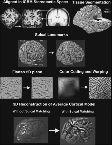 FIGURE 2. Steps in cortical pattern-matching algorithm. Raw images are first globally aligned to a standard template. Tissue classification partitions the image into gray and white matter and cerebrospinal fluid based on voxel intensity. A three-dimensional (3D) cortical model is extracted from each scan, and sulci are traced and labeled directly on the surface model. A geometric flattening process transforms the cortical model into two-dimensional (2D) space with retained sulcal landmarks. A color-coding system with intensities of the red, blue, and green corresponding proportionally to the x, y, z location of the three-dimensional cortical model plot the original coordinates onto the flat map. A warping technique uses the sulcal landmarks to constrain one cortical region onto another. The result produces an averaged cortical model for each group across subjects. ICBM, International Consortium for Brain Mapping; CENT, Central Sulcus; SFS, Superior Frontal Sulcus; STS, Superior Temporal Sulcus; SYLV-Sylvian Fissure. (See the color insert.) |
Large-Deformation High-Dimensional Brain Mapping
HDBM-LD is a diffeomorphic mapping technique that analyzes subtle shape variations in subcortical brain structures.17,29,37 This method has been applied to such enclosed structures as the hippocampus in epilepsy.25,26 In this method, the typical brain structure is represented as a template and its variabilities determined by probabilistic diffeomorphic transformations applied to the template. A diffeomorphic transformation produces a map between topologic spaces that is constrained by laws of continuum mechanics while allowing all data points independent freedom to match. This allows the geometric properties of the neuroanatomic substructures to be preserved. The algorithm begins with semiautomatic segmentation of the hippocampus. Individuals with expert anatomic knowledge first manually segment a template hippocampus.25 Brain images from target scans are then globally aligned to the template image with standard landmarks from a coordinate system such as that of Talairach and Tournoux.47a Hippocampal-specific landmarks such as the head and tail define the long axis of the hippocampus in the target scan. Several additional landmarks are placed in cross sections along the axis. Using these manually defined hippocampal
boundaries, a mapping algorithm generates transformation fields from template images to the target images, thus automatically defining the hippocampus. More important, the diffeomorphic transformation fields and the matrices derived from them contain information defining the composite shape and volume of the structure. Statistical tests can be applied to determine the degree of shape and volume change between groups and within individuals over time. The initial steps of defining the brain structure of interest in the template image and landmarks in the target images require knowledge of neuroanatomy. Once the template structure has been delineated and target boundary points have been chosen, this algorithm relies solely on the transformation to apply the neuroanatomic information to a large number of individual target scans.
boundaries, a mapping algorithm generates transformation fields from template images to the target images, thus automatically defining the hippocampus. More important, the diffeomorphic transformation fields and the matrices derived from them contain information defining the composite shape and volume of the structure. Statistical tests can be applied to determine the degree of shape and volume change between groups and within individuals over time. The initial steps of defining the brain structure of interest in the template image and landmarks in the target images require knowledge of neuroanatomy. Once the template structure has been delineated and target boundary points have been chosen, this algorithm relies solely on the transformation to apply the neuroanatomic information to a large number of individual target scans.
Anatomic Surface Modeling
This method uses surface-based mesh modeling combined with surface-based statistics to map the three-dimensional profile of an enclosed structure such as the hippocampus or ventricle.33,52 Images are first linearly aligned and manually registered to the average template stereotaxic space (Fig. 3). A standard neuroanatomic atlas is used as a guide to manually segment the hippocampus. Hippocampal models are then delineated in continuous coronal brain MR sections, including the hippocampus proper, dentate gyrus, and subiculum. Based on the use of interactive segmentation software, anatomic landmarks are followed by viewing images in all three orthogonal planes simultaneously. An anatomic mesh modeling method is used to match equivalent hippocampal surface points obtained from manual tracings across subjects and groups. Three-dimensional parametric surface mesh models are generated from manually segmented hippocampal tracings. This allows one to match the digitized points in the parametric surface model in each brain volume, and these corresponding surface points can be compared statistically in three dimensions. This surface matching method also allows the calculation of average hippocampal morphology across individuals belonging to a group and the variance among corresponding surface points relative to group averages.
Related posts:


Stay updated, free articles. Join our Telegram channel

Full access? Get Clinical Tree


