Indications for continuous electroencephalogram monitoring (Taken from Friedman D, Claassen J, Hirsch LJ. Continuous electroencephalogram monitoring in the intensive care unit. Anesth Analg 2009; 109: 506–523 with permission from the publisher. https://insights.ovid.com/pubmed?pmid=19608827)
Further, recent studies have suggested that continuous EEG can be used to detect ischemia at a reversible stage and at the moment that starts. Quantitative EEG analysis with trending of alpha/delta ratio may be helpful for this looking particularly promising as a method for real-time ischemia detection [5], and we also provide a review of other signal processing techniques that support qEEE.
5.2 Continuous EEG for Detection of Nonconvulsive Seizures and Status Epilepticus
The incidence of status epilepticus in the USA is about 150,000 cases/year [6]. In general terms, seizures and status epilepticus (SE) are divided into convulsive (with prominent motor symptoms) and nonconvulsive types (absence of motor symptoms).
Based in experimental experience, when a convulsive seizures persist longer than 5 min, treatment should be started, and if convulsive status lasts beyond 30 min, more aggressive treatment should be implemented to prevent irreversible brain damage (including neuronal injury, neuronal death, and dysfunction of neuronal networks) [7].
Nonconvulsive seizures are electrographic seizures with little or no overt clinical manifestations, so EEG is necessary for detection. There is limited information regarding when to start treatment in nonconvulsive status epilepticus, but for operational purposes, it is suggested to start treatment after a prolonged nonconvulsive seizure lasting longer than 10 min and to escalate therapy when lasting >60 min to avoid long-term consequences [8].
Nonconvulsive seizures and nonconvulsive status epilepticus are increasingly recognized as common occurrences in the ICU. In many patients who present with convulsive SE, electrographic seizures can persist even when convulsive activity has ceased, and cEEG becomes an important diagnostic tool to evaluate for these subclinical seizures. A wide range of comatose patients 8–48% may have NCSz depending of the type of patients studied [4]. In a prospective study of 164 patients with convulsive SE, DeLorenzo et al. found 48% to have NCSz, and 14% to have NCSE on cEEG 24 h after convulsive SE had stopped. These patients were comatose after their convulsive SE and had no clinical signs of convulsive activity. Therefore, cEEG monitoring is an essential diagnostic tool on any patient who does not quickly regain consciousness after controlling convulsive seizures to guide further treatment. The most common reason for performing cEEG in the ICU is to detect NCSz or NCSE.
A prolonged “post-ictal state” following generalized convulsive seizures or other clinically evident seizures. If a patient is not showing clear signs of improved alertness within 10 min.
A prolonged reduction of alertness from a spontaneous neurologic insult or operative procedure.
Unexplained acute onset or fluctuating levels of impaired consciousness or coma.
Impaired consciousness with myoclonus of facial, axial muscles or nystagmoid eye movements.
Clinical paroxysmal events that rise concerns for seizures such episodic blank staring, aphasia, automatisms (lip smacking or fumbling with fingers), and perseverative activity.
Other paroxysmal spells such posturing, rigidity, tremors, agitation, or sudden changes in pulse or blood pressure without an obvious explanation are also susceptible to be monitored because none of these signs are highly specific of seizure activity and they are often found under other circumstances in critically ill patients.
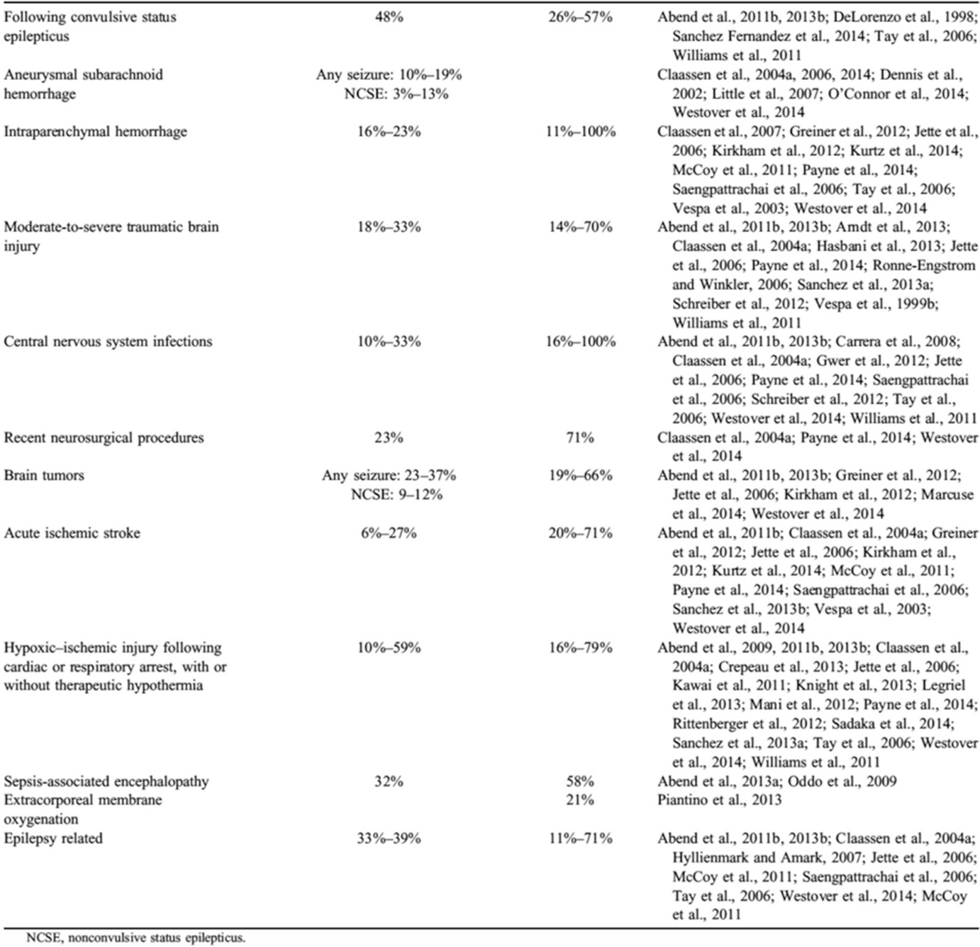
Common neurological, medical, and surgical conditions associated with high likelihood of recording seizures on critical care continuous EEG (Taken from Herman ST, Abend NS, Bleck TP, et al. Consensus statement on continuous EEG in critically ill adults and children, part II: personnel, technical specifications, and clinical practice. J Clin Neurophysiol 2015; 32: 96–108, with permission from publisher. https://www.ncbi.nlm.nih.gov/pmc/articles/PMC4434600/)
Nonconvulsive seizures and NCSE are also associated with other signs of neurological injury such increased intracranial pressure, increased edema and mass effect, changes in tissue oxygenation, and increases in lactate/pyruvate ratio and glutamate suggesting that NCSz play a role in secondary neurological injury. Therefore, early detection of seizures with cEEG and its treatment is thought to be essential to decrease mortality and improve neurological outcome of these patients [12–17].
As of today, the impact of early diagnosis and treatment of NCSz on outcome has not been established. However, it has been associated with increased mortality and poor neurological outcome [10, 18, 19].
5.2.1 Basic Principles of Quantitative EEG for Seizure Detection
The advantages of qEEG technique are mainly due to its capacity of synthesizing extensive raw EEG data and clear presentation of the results, making this technique easy to learn and interpret even by people not specifically trained in electroencephalography [20].
The qEEG should never replace expert review of raw EEG, but it does allow for a quick visualization of up to several hours of EEG data on a single screen display (1–4 h of qEEG as opposed to 10 s of raw EEG with conventional EEG review) expediting seizure detection, localization, frequency, and response to treatment [21, 22]. The qEEG can also reveal at a glaze subtle background asymmetry, changes in state, reactivity, and rhythmic or periodic patterns that may fluctuate over the course of several hours.
Fast Fourier transformation spectrogram (FFT spectrogram or color spectrogram). The mathematical technique that breaks up the EEG signal into its components is explained later in this chapter. This spectrogram shows the time in the horizontal (x) axis and frequency in the vertical (y) axis (0–20 Hz), and the color (z) axis is power. The power is a calculation of the total “amount” of a given frequency (based on amplitude) and is represented on a color scale where the highest power is white and the lowest is dark blue (Fig. 5.3, fifth and sixth panel/row).
Rhythmicity spectrogram: It highlights (in dark blue) the rhythmic activity associated with seizures at a given frequency. The color (z) axis in this panel represents the amplitude (Fig. 5.3, third and fourth panel).
Amplitude integrated EEG (aEEG): Displays minimum and maximum amplitude of all background activities. Seizures are represented by an increase in baseline amplitude (Fig. 5.3, last panel).
Asymmetry, relative spectrogram: This spectrogram shows the difference in frequency between homologous electrodes of both hemispheres. Asymmetry is indicated in red for right-weighted and blue for left-weighted asymmetry (Fig. 5.4, fifth panel).
Absolute asymmetry index: The absolute asymmetry index shows total asymmetry in yellow, which is calculated by comparing at each pair of homologous electrodes and summing their absolute values to give a total asymmetry score; this only can be positive and upward for asymmetry in any frequency or direction. The green relative asymmetry shows laterality; downgoing indicates more power on the left and upgoing indicates more power on the right (Fig. 5.4, sixth panel).
Peak envelope: This trend shows amplitude (y-axis) of EEG within the 2–20 Hz frequency range. Seizure activity often occurs within this frequency range, so is helpful for seizure review (Fig. 5.3, second panel).
Spike detection: This trend shows the rate of spikes detected per 1 s epoch for the left hemisphere and right hemisphere (Fig. 5.3, seventh and eighth panel).
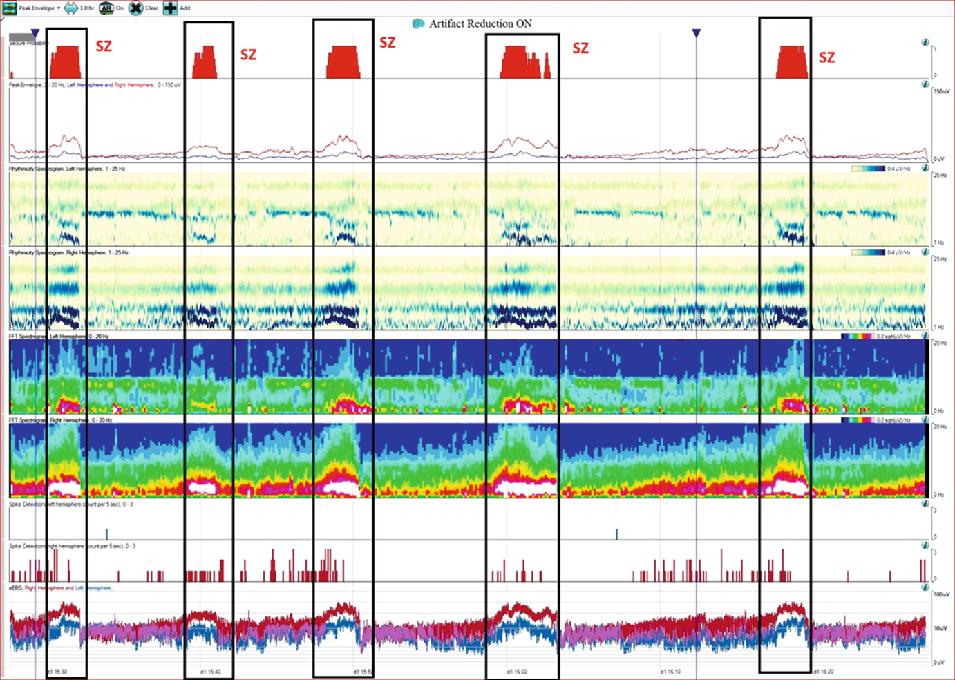
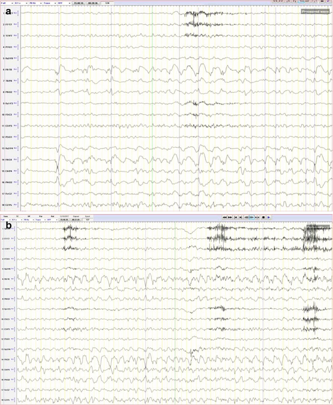
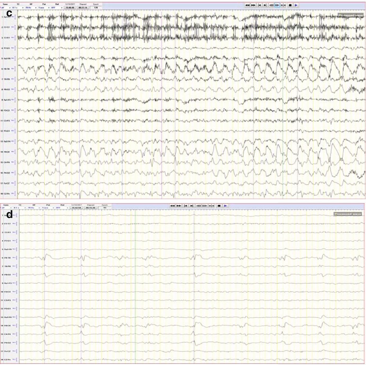
Case 1.This trend panel shows one hour of qEEG in a 70-year-old man with a right hemisphere brain tumor. Four nonconvulsive seizures and one manifesting with focal motor activity were recorded (labeled as Sz), originating from the right hemisphere. The following qEEG includes different panels (rows). FFT spectrogram of the left and right hemisphere (fifth and sixth panels) shows intermittent bursts of increased power in all frequencies on the right hemisphere with the highest power at lower frequencies (white area). These intermittent bursts of increased power represent seizures, although review of the raw EEG at that point is necessary to confirm this (see a–c). The rhythmicity spectrogram of the left and right hemisphere (third and fourth panel) shows a dark blue band at the frequency of the rhythmic pattern consistent with seizures. Overall amplitude gradually increases during seizures, as can be seen on the amplitude-integrated EEG (aEEG) tracing on the bottom (last panel). The amplitude is higher over the right hemisphere with each seizure (red band). Coinciding with the gradual increase of amplitude, the spike detection panels (seventh and eighth panel) shows progressive increase of periodic discharges (PLEDs) on the right hemisphere (see d). (a) Raw EEG showing evolving seizure as a rhythmic sharply countered delta activity with maximum electronegativity in the right centro-parietal region (timebase: 30 mm/s). (b) Progression of the seizure (+20 s) now with more admixture of frequencies over the right hemisphere (timebase: 30 mm/s). (c) Progression of the seizure (+35 s). On the left hemisphere, muscle artifact is mainly seen over the left temporal chain coinciding with clinical onset of left facial clonic activity (timebase: 30 mm/s). Note the increase EMG activity (d) Interictal EEG showing periodic lateralized epileptiform activity over the right hemisphere with maximal electronegativity in the right centro-parietal region (timebase: 30 mm/s)
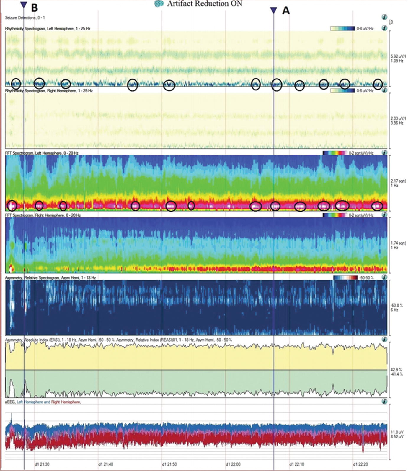
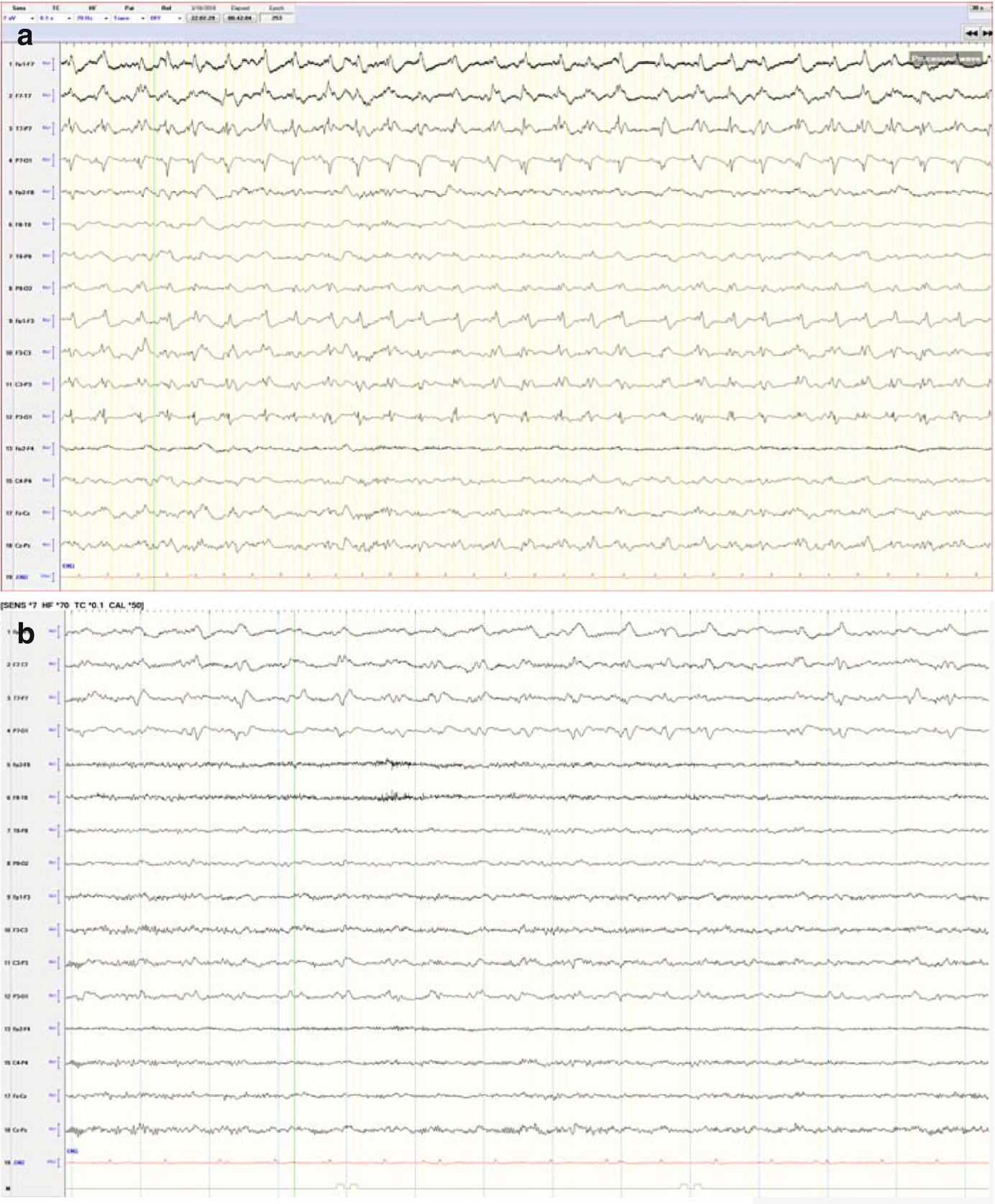
Case2. One hour of qEEG in a 58-year-old woman with left hemispheric stroke. FFT spectrogram (third and fourth panel) shows a continuous asymmetry with greater power in all frequencies on the left hemisphere and with this difference most notable at lower frequencies (white and red area). Notice that coinciding with this white area, the raw EEG shows a cyclic pattern of periodic lateralized epileptiform discharges (PLEDs) arising from the left hemisphere averaging ~1.5 Hz every 2 min (a). The same rhythmic and periodic activity is seen in the rhythmic run detector panel or rhythmicity spectrogram on the left hemisphere (first and second panel) that shows this activity as a dark band at lower frequencies. The asymmetry is also well appreciated in the relative asymmetry index tracing (sixth panel), where a persistent green area below zero is seen with greater power on the left hemisphere (downgoing). The asymmetry spectrogram also shows a continuous asymmetry with greater power on the left (dark blue). The amplitude-integrated EEG (aEEG) trend is shown in the seventh panel where the tracing is a band (red = right, blue = left) with width, maximal and minimal amplitudes given for each EEG epoch. In this case, the amplitudes are higher over the left hemisphere. (a) Raw EEG at point A showing a segment of recording showing left PLEDs averaging ~1.5 Hz (timebase: 30 mm/s). (b) Raw EEG at point B showing a segment of recording with less frequent (~0.5–1 Hz) and poorly formed periodic left hemispheric epileptiform discharges (timebase: 30 mm/s)
From the top to the bottom: Seizure probability panel, peak envelope, 2 rhythmicity spectrograms, 2 color spectrograms, 2 spike detection panels (upper row corresponds to the left hemisphere and the lower row to the right respectively), and the amplitude EEG (aEEG) where the left hemisphere is represented in blue and the right in red.
5.3 Continuous EEG for Detection of Cerebral Ischemia
The use of cEEG monitoring to monitor patients for cerebral ischemia detection is based on the rational that electrical brain activity is affected by any variation of cerebral perfusion. Studies from intraoperative EEG monitoring and animal models have shown that EEG changes occur within 5 min of acute cerebral ischemia. The early detection of these changes in the EEG tracing would be superior to current imaging methods and to clinical examination especially if the patient is paralyzed, sedated, or is encephalopathic.
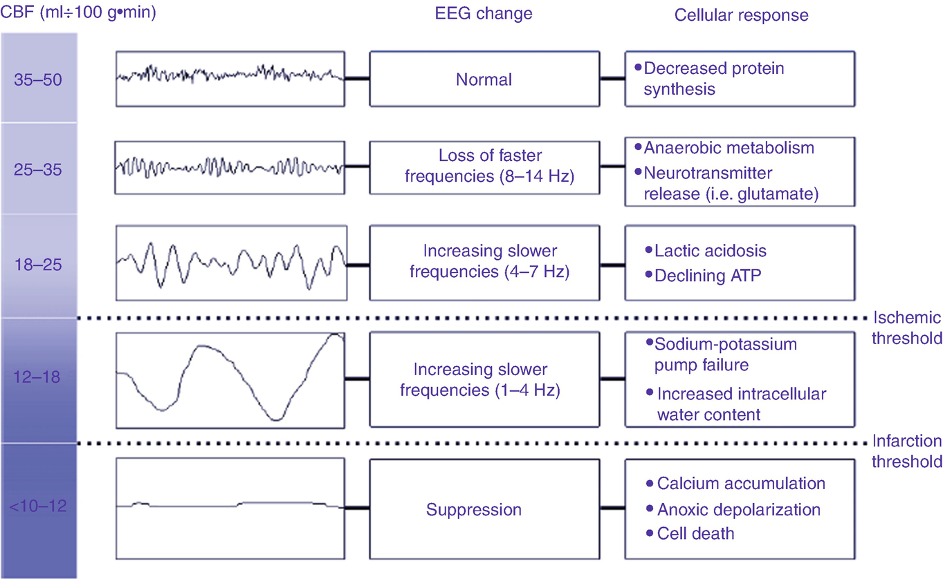
The relationship of cerebral blood to the encephalogram and pathophysiology (Taken from Foreman B, Claassen J. Quantitative EEG for the detection of brain ischemia. Crit Care 2012; 16: 216 with permission from Springer Nature)
Retrospective studies have shown that cEEG monitoring, particularly qEEG trends, can identify ischemia at reversible stages during the process of vasospasm in subarachnoid hemorrhage patients and, therefore, have a time frame window (of hours to days) for initiation of therapy to prevent irreversible infarct [3, 5].
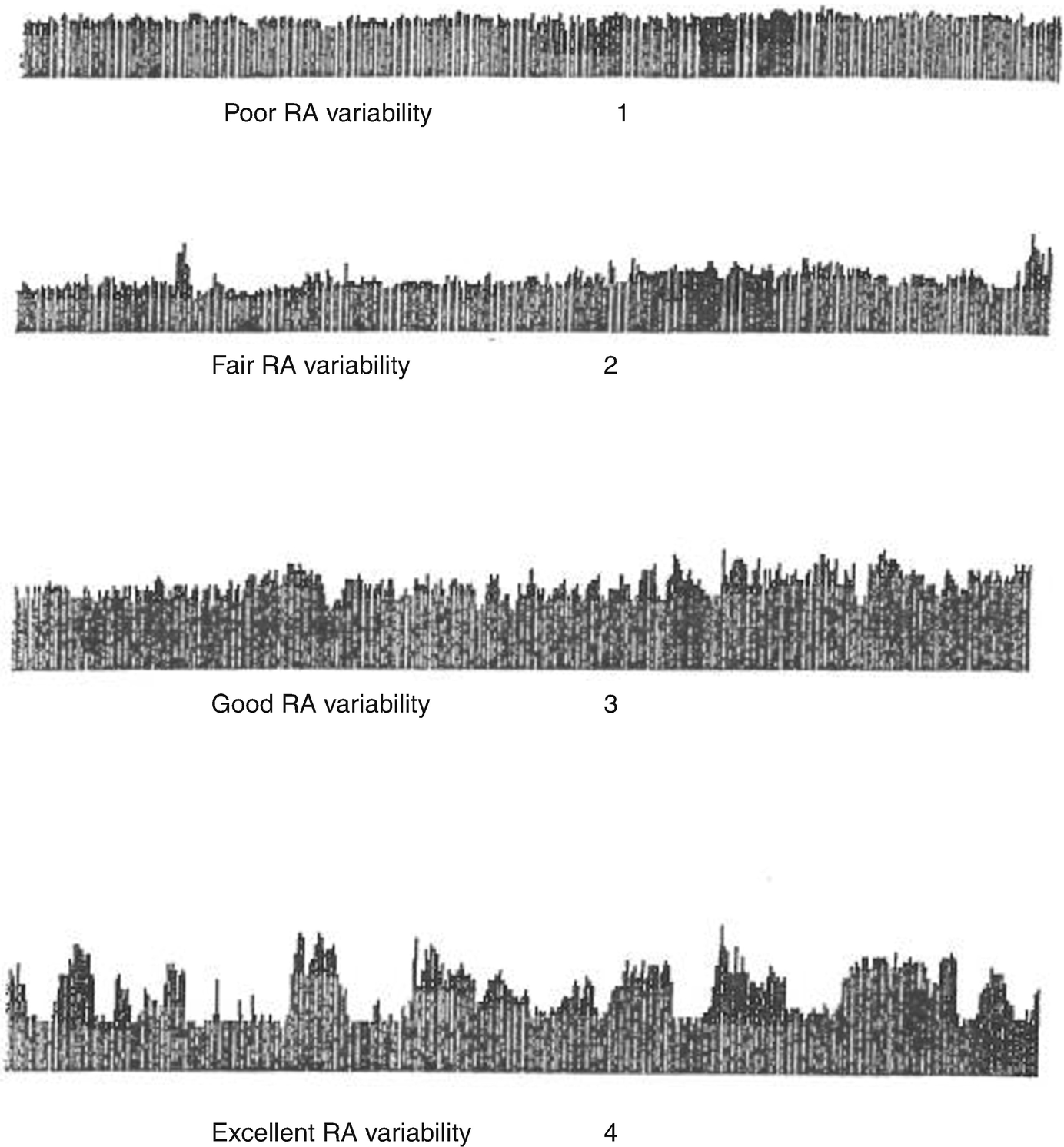
Relative alpha variability (RAV) visual scale (Vespa PM 1997) RAV is calculated as the ratio of theta-alpha power (6–14 Hz) to total power (1–20 Hz) (Taken from Vespa PM, Nuwer MR, Juhasz C, Alexander M, Nenov V, Martin N, Becker DP. Early detection of vasospasm after acute subarachnoid hemorrhage using continuous EEG ICU monitoring. Electroencephalogr Clin Neurophysiol 1997; 103: 607–615 with permission from the publisher)
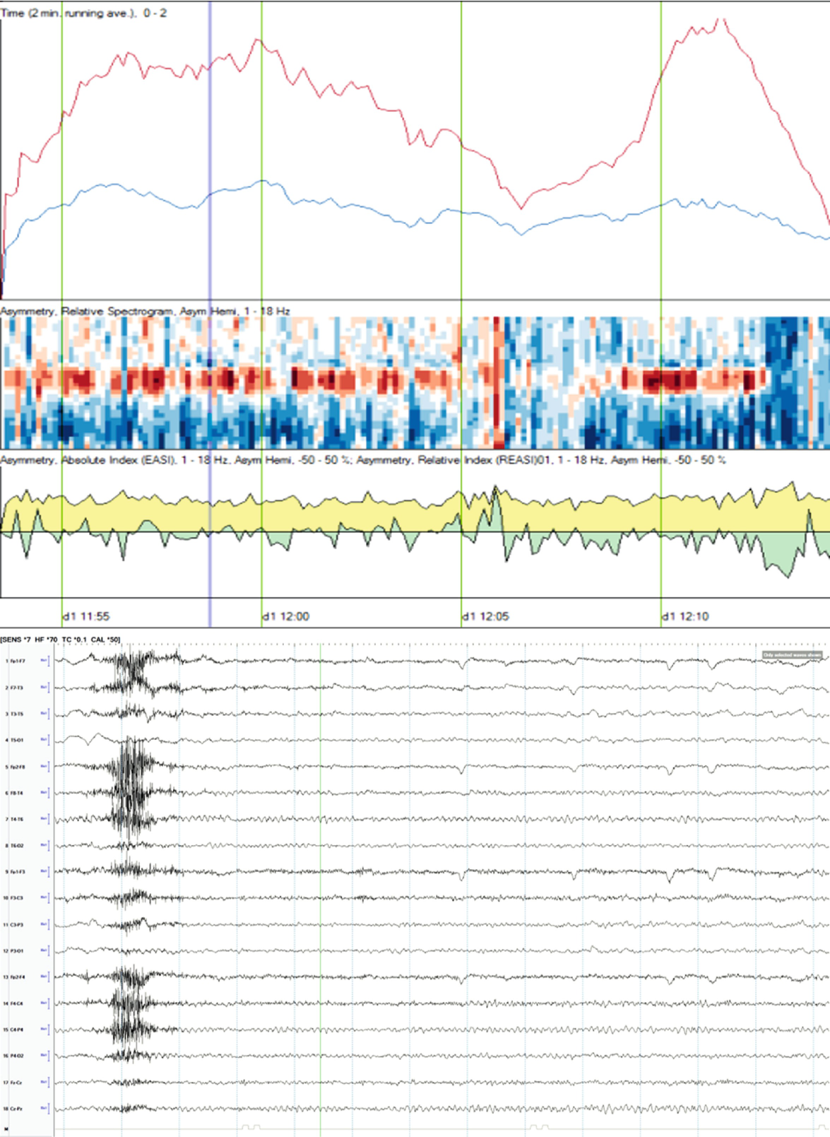
qEEG: Unilateral ischemia and basics of symmetry measures. Same patient illustrated in Fig. 5.4, a 58-year-old woman with left hemispheric stroke. Ischemia on alpha-delta ratio∗: since alpha frequencies decrease and delta increase with ischemia, the ADR is used to magnify this difference when looking for ischemia. The upper panel shows the ADR on each side (red = right). Note that the ADR is persistently higher on the right, suggesting ischemia on the left. The absolute asymmetry index shows total asymmetry in yellow, which is calculated by comparing at each pair of homologous electrodes and summing their absolute values to give a total asymmetry score (only an upward deflection). The green relative asymmetry tracing indicates laterality (downward deflection indicates more power on the left and upward on the right). Note in this case that the green tracing is variable and usually downward, indicating more power on the left. Asymmetry spectrogram shows asymmetry at each frequency (1–18 Hz) averaged over the entire hemisphere. Red means more power on the right in a particular frequency. In this case, higher frequencies are greater on the right (red), and slower frequencies (~4 Hz) are greater on the left (blue). ∗ADR is calculated as the ratio of alpha power (8–13 Hz) to delta power (1–4 Hz). Raw EEG: note the attenuation of faster frequencies in the left hemisphere, including the alpha rhythm that is well developed on the right. There is continuous left hemispheric slowing (timebase: 30 mm/s)
5.4 Continuous EEG for Assessment of Encephalopathy and Prognostication
Coma is a state of impaired consciousness that can range from confusion to complete unresponsiveness.
Continuous EEG monitoring in patients with altered level of consciousness can be used to assess depth of encephalopathy or coma, help determine the etiology, provide prognostic information, detect nonconvulsive seizures, and help to differentiate coma from other states of unresponsiveness (e.g., locked-in syndrome, catatonia).
Because the EEG of comatose patients is dynamic, continuous EEG is preferred to serial EEGs to avoid missing favorable prognostic factors and seizures.
Unfavorable prognostic factors include isoelectric pattern, burst suppression pattern, periodic patterns, and electrographic seizures. Favorable prognostic features include background continuity, spontaneous variability, reactivity to stimulation, and presence of normal sleep patterns. Ensuring accurate clinical information regarding the medications being administered is essential because many medications can produce EEG changes that are identical to changes seen with brain injury [26–28].
The different EEG patters in encephalopathy and coma are nonspecific of etiology; however, some features help to determine if the alteration of consciousness is the result of a diffuse physiological brain dysfunction related to systemic etiologies (sepsis, renal and/or hepatic dysfunction, intoxication, etc.) or related to primary brain disorders (encephalitis/meningitis, diffuse cerebral injury from trauma, anoxia/hypoxia, structural lesions or ischemia, etc.). Largely, prognosis depends on the type of the neurological insult.
A prospective study of 236 patients found that NCSE is an under-recognized cause of coma, occurring in 8% of all comatose patients without signs of seizure activity. This supports that cEEG should be included in routine evaluation of comatose patients even when clinical seizure activity is not present [29].
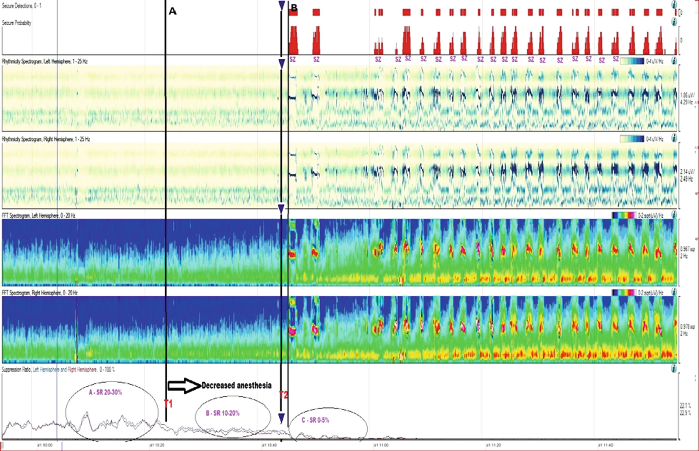
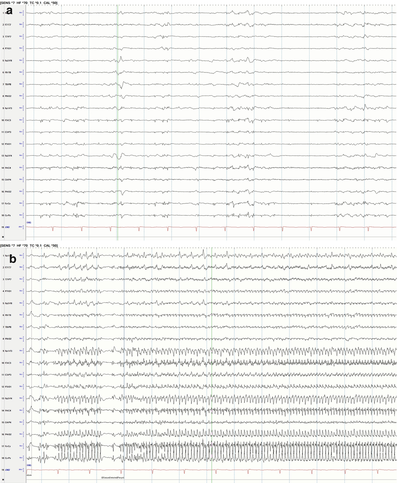
Long-term trends: Midazolam coma, wearing off anesthetic and suppression-burst pattern. qEEG of a patient who was being treated with midazolam for refractory status epilepticus. The suppression ratio was initially ~20–30%. At point T1, anesthesia dose was gradually reduced being a decreased in suppression ratio to 10–20% after T1 and further to 0–5% soon after T2. After point T2, there were frequent seizures, which are easily identified in the FFT spectrogram and rhythmicity spectrogram. This provides evidence that anesthesia at 20–30% suppression was enough helping control seizures with recurrence of seizures after weaning it. (a) Raw EEG at point A: short bursts of cerebral activity on a background of suppression (burst-suppression pattern) (timebase: 30 mm/s). (b) Raw EEG at point B: evolving electrographic seizure characterized by paroxysmal fast activity maximal at midline regions (timebase: 30 mm/s)
5.5 Quantitative EEG Methods
Quantitative EEG (qEEG) refers generally to the analysis of EEG signals using computational methods. This extends the traditional visual analysis of EEG to include quantitative time domain, frequency domain, and time-frequency domain methods applied to individual and multiple EEG recordings. In this section we will provide a review of some of the most common signal analysis methods that have been applied to EEG as well as discuss opportunities for integrated multi-channel analysis using emerging signal processing methods for feature extraction, classification, and clinical decision support. This review is not intended to be comprehensive, but provides a good overview of selected time and frequency domain methods and techniques and should provide a good general introduction.
5.5.1 Data Acquisition
The EEG signal is a time domain waveform that is acquired using a data acquisition system and is transformed to sampled digital data. The sampling rate (number of samples per second) is in the range of 200–10,000 samples per second depending on the application. The sampling operation transforms the continuous-time and continuous-valued (analog) EEG waveform x(t) to a discrete-time signal (time-series) of the form x(n), where n is the index of the time samples, tn = nts and ts is the sampling time. At the time of acquisition, high-pass and low-pass filters are implemented to eliminate DC and very low and high frequency content in the EEG signals. The low-pass filter can also provide anti-aliasing protection so that the frequency content is the acquired signal and the sampling rate are consistent. Further, because the data is stored in digital format, the continuous values of the waveform are quantized into a digital (binary) data format. The binary data format is characterized by the resolution of the quantizer that is determined by the number of bits that are used to represent the data. If there are N-bits in the data representation, then the range of the data is quantized into 2N different bins. Generally, N is on the order of 16, 32, or 64 in modern day EEG acquisition systems, so that for all practical purposes, we can assume the time-series x(n) is continuous-valued. Next we represent a collection of methods for feature extraction, an approach to transform raw input data into lower dimensional data sets for quantitative analysis. EEG, like most other physiological signals, is nonstationary meaning that in different time periods where the time series is studied, the signal may have different properties and characteristics. Hence, feature extraction for nonstationary time series requires a windowed analysis, where the total length of the recorded time series is divided into smaller time periods (windows) for analysis. Hence it what follows, for each analysis method applied to the time-series data, it is assumed that we are working with one window of data.
Another important issue that must be considered is the impact of artifacts on the computational methods being used for feature extraction. Scalp EEG is easily contaminated with many artifacts including those that are biological (e.g., eye movements) and those that are not (e.g., changes in recording electrode impedance). Eye movements, e.g., REMs, can cause serious artifacts called ocular artifacts. Ocular artifacts contaminate the EEG signal because there is a potential difference of a few millivolts between the cornea and retina, the former being positive with respect to the latter and thus the eyes can be considered an electrical dipole. Movement of the eyeballs or eyelids causes a change in the electric field that is picked up by electrodes in their vicinity, mostly in the frontal EEG channels. Other biological artifacts include EKG and EMG artifact. EKG artifact results from contamination of the EEG by the electrical activity of the heart, where EMG is a high frequency—low amplitude signal induced by muscle activity.
In windowed time-series analysis, we decompose the total signal into epochs, and the objective is to analyze each epoch and then use the epoch-by-epoch analysis to identify changes in the EEG that can be related to biological changes. A good example is when EEG is used for sleep scoring, where the traditional epoch for visual analysis is usually 30 s. Each epoch is given a label that refers to a particular sleep state and because the signal is nonstationary, usually when more than half of the epoch is classified as a particular state the entire epoch is labeled with that state. Suppose movement occurs at a given time and lasts for 20 s or more, this can then have a significant impact on how that epoch is labeled. One way to deal with the artifact is to detect the occurrence and then eliminate the epoch from further consideration.
Because artifacts can mask relevant features in the EEG signal, the artifact components must be removed prior to any analysis. Ocular artifacts seem to be the most serious problem in EEG analysis and are very difficult to remove. The amplitude of ocular artifacts is much higher than the scalp signals, but the frequency is lower. Unlike movement artifacts, ocular artifacts are generally present, so rejection may cause loss of information. Algorithms for removing ocular artifacts have been developed, and the classic algorithm is a regression-based method where the EOG signal must be measured and the propagation factors between EOG and EEG channels must be defined.
Other methods for removing ocular artifacts are component-based methods that assume the EEG signal is a linear mixture of the scalp signal and the artifact signal, i.e., S = W·X, where S is the signal source (scalp and artifact components), X is the measured signal, and W is the mixing matrix. Once the mixing matrix W is determined, the signal source S is calculated, and then the artifact components are identified and isolated by setting the rows of S to zero. The cleaned EEG signal is then given by X∗ = W−1·S∗, where X∗ is the cleaned EEG and S∗ is the signal source in which the artifact components have been removed. The calculation of the mixing matrix W leads to two different component-based methods based on either principal component analysis (PCA) or independent component analysis (ICA). PCA, which is a feature reduction techniques, will be discussed later in this section.
5.5.2 Time Domain Methods
The simplest time domain method for feature extraction is to compute the statistics of the time-series data. Given a time series  the mean of the time series is,
 and the variance (var) of the time series is
  ,where the standard deviation (SD) is equal to the square root of the variance.


