Electroencephalogram Mapping and Dynamic Analysis
Peter K. H. Wong
Fernando H. Lopes da Silva
Introduction
In its simplest use, mapping of the scalp electroencephalogram (EEG) provides a convenient display of instantaneous scalp topography, usually that of resting background or interictal spike activity. In more complex forms, the scalp EEG data are subjected to mathematical manipulation as prescribed by a theoretical model. The result is a variety of parameters capable of characterizing the input data, albeit always within limitations imposed by the model. In between these two approaches is a large variety of methods using quantitative analysis.
In the clinical arena of epilepsy diagnosis, EEG analyses seek maximally to extract information pertaining to the epileptic discharge so as to facilitate the understanding of the underlying focus and its current and future behavior. The final purpose is then to use such information for earlier and more accurate diagnosis, which, in turn, can facilitate appropriate treatment and management. This is of particular importance when surgical resection is contemplated.
With spike discharges, the routine EEG tracing provides good visual information regarding spike morphology, scalp localization, and temporal changes (see Chapter 73). It is generally accepted that more useful information might be available but undiscovered. This drives the search for better and more productive display techniques, usually based on computer software algorithms. However, there is no consensus on what technical approaches are useful or acceptable. It is appropriate to observe that newer algorithms and theoretical models tend to be viewed with skepticism. This view has some valid basis, in part generated as a reaction to schemes that purport to make instant clinical diagnoses of various kinds based only on scalp recordings, without the need for clinical assessment. Such computerized diagnostic “aids” have been proposed for differentiating depression from dementia, for example. One is well advised to exercise caution with any such device.
We hope that by increasing the understanding and knowledge base of prospective users, choice of methodology and utilization can be made based on sound neurophysiologic considerations. Toward this end, this chapter reviews selected techniques and results.
Methodology
General Aspects: Electroencephalography and Magnetoencephalography
Electroencephalographic signals reflect the dynamics of the electrical activity generated by populations of neurons (see Chapter 72). This activity is caused by ionic currents flowing through neuronal (and glial) membranes between the intra- and the extracellular space. These signals can be measured at a considerable distance from the sources when two conditions are satisfied: (1) the responsible neurons are regularly organized in space and (2) they are activated in a rather synchronized fashion. As regards the first condition, the cortical neurons form the main sources of EEG potentials because they are arranged in palisades perpendicular to the cortical surface and are activated by synapses distributed in a regular way along their soma-dendritic membranes. According to this spatial organization, their synaptic activation causes the generation of potential fields with a dipole layer configuration. The second condition, synchronization of neuronal populations, is important because in this way, potential fields can be generated that are sufficiently strong to attain the necessary signal-to-noise ratio to be recordable at a distance. The main factor responsible for the synchronous activity of populations of neurons also has a structural basis. It consists of the fact that the neurons within these populations form interlocked networks through excitatory and inhibitory synaptic connections. These populations of interconnected neurons form the macroscopic sources of EEG signals. The neuronal ionic currents not only generate electric fields; they also give rise to magnetic fields. The latter constitutes the magnetoencephalogram (MEG) (see later discussion and Chapter 78).
Although EEG and MEG are caused by the same elements, in practice the two types of signals differ: (1) The EEG is a relative measurement needing a reference electrode; this does not apply to the MEG; (2) the MEG is a signal that consists of the magnetic fields oriented perpendicular to the skull that are caused by current dipoles tangential to the cortical surface, whereas the radial components do not contribute significantly to the MEG signal; the EEG signal is a measure of both tangential and radial components; (3) the MEG pattern of activity is more focal than the corresponding EEG pattern because the former is much less dependent on variations in resistivity of the volume conductor.
Sampling in Time and Space
Electroencephalographic signals are continuous variations of electrical potential as a function of time and space. The same applies to the variations of magnetic fields that form the MEG signals. In practice, these signals must be digitized to be quantified and analyzed. First we consider this question in terms of the variable time. This implies that the signals have to be sampled at a certain rate and that their amplitude has to be quantified. These operations must take place in such a way that all important information contained in the signals is preserved. Accordingly, the Nyquist sampling theorem has to be satisfied: If the signal has a frequency spectrum with an upper limit fN, the signal should be sampled at a frequency at least equal to
2fN. This means that care should be taken that the signal does not contain frequency components >fN to avoid aliasing, that is, all frequency components >fN should be zero. Thus, before sampling, all frequency components >fN should be eliminated by appropriate filtering. For most EEG-MEG signals, a quantitization into 4096 amplitude levels (i.e., 12-bit precision) is appropriate and commonly available. In practice, however, the Nyquist criterion, although a minimally necessary condition, is not sufficient for displaced signals, and a sampling frequency of >3fN should be used.
2fN. This means that care should be taken that the signal does not contain frequency components >fN to avoid aliasing, that is, all frequency components >fN should be zero. Thus, before sampling, all frequency components >fN should be eliminated by appropriate filtering. For most EEG-MEG signals, a quantitization into 4096 amplitude levels (i.e., 12-bit precision) is appropriate and commonly available. In practice, however, the Nyquist criterion, although a minimally necessary condition, is not sufficient for displaced signals, and a sampling frequency of >3fN should be used.
Another aspect of the temporal properties of EEG-MEG signals that has to be taken into consideration here is that the statistical properties of these signals can change as a function of time (i.e., nonstationary properties). However, they can be subdivided into representative segments, or epochs, that are quasistationary. A precise definition of the duration of these epochs cannot be given in general terms because it depends on the subject’s condition. Nevertheless, it has been shown20,30 for EEG signals recorded in a general population that 90% had time-invariant properties for epochs of about 20 seconds, whereas <75% remain time invariant after 60 seconds. This means that it is, in general, safe to choose epochs with a duration of 10 to 20 seconds to avoid deviations from stationary behavior.
Sampling in space must obey the same general rules as sampling in time. However, it is much easier to grasp the meaning of a frequency component in the time domain than one in the spatial domain. What is the spatial frequency of a given EEG signal? This can be accounted for by considering a model of a source within a volume conductor, which will cause a potential distribution at the surface of the conductor. Using Fourier analysis, we can represent this potential distribution as a spectrum of spatial frequencies. The sharper the potential distribution, the higher are the corresponding spatial frequencies. It is important to know the upper limit of this spatial frequency spectrum to estimate how sampling in space should take place in an optimal way. If the sampling in space is not appropriate, an aliasing error will be introduced. In general terms, the traditional 10–20 system can be sufficient to sample in space most potential distributions that are rather widespread and smooth, but not those distributions that are highly focal and change abruptly with distance. Some practical questions posed by sampling this kind of potential distribution, in which a high spatial resolution has to be achieved, are discussed later.
Two other fundamental issues need to be further understood—volume conduction and the “inverse problem.” The former is a physical phenomenon that smears or blurs the EEG signal as a result of the different layers of tissues interspersed between source and electrode (brain, cerebrospinal fluid, skull, muscle, fat). The result is added uncertainty about the EEG source. The “inverse problem” refers to the process of inferring the source characteristics from the recorded EEG signal. Fundamentally, this problem has no clear or unique mathematical solution, and is the reason for the general skepticism about dipole localization methods (DLMs; see later discussion). Certain mathematical simplifications that are implicit (e.g., the number of sources, the configuration being small and localized rather than as a layer) might not be clinically appropriate. Experience with application to known problems (e.g., somatosensory-evoked potentials, visual-evoked potentials, known epileptogenic lesions) allows some general understanding of its capabilities and limitations, which can guide its use under certain circumstances.
The detection of specific signals in the background EEG, whether occurring spontaneously, such as epileptiform spikes, or evoked by sensory stimuli, is not only an important general problem in electroencephalography, but it is also relevant for the estimation of the parameters of the equivalent dipole sources. This is a classic problem of detection of signals in noise. The background EEG represents the noise term. To optimize the detection, it is important to know the statistical properties of the noise, that is, the background EEG. Knowledge of these statistical properties is necessary to estimate the confidence limits of equivalent dipole parameters and to design optimal noise filters to improve the signal-to-noise ratio. The spatiotemporal covariance matrix of the background EEG differs with frequency band. For the frequency bands 5 to 8 Hz and 13 to 30 Hz, it was found experimentally that the variance is a function of electrode distance that is compatible with a generator model consisting of random dipoles with a spherically symmetric distribution. However, for the alpha (9 to 12 Hz) frequency band, such a distribution is not adequate, and a localized model consisting of one or more clustered dipoles has to be assumed. These estimates of the statistical properties of the background EEG have practical implications because they allow the construction of maximum likelihood estimators for evoked potentials/magnetic fields based on the spatiotemporal covariance matrix of the background signals.7
High-Resolution Electroencephalography and Magnetoencephalography
The condition in which the highest possible spatial frequencies are achieved can be represented by a source consisting of a radial dipole situated in the cortex, that is, close to the surface of the volume conductor. This may correspond to the source of an epileptiform spike located in the cortex. If one uses the traditional 10–20 system (interelectrode distance of about 4.5 cm), the aliasing error in such a case is 6%. To reduce this error to the more adequate level of 1%, one must reduce the interelectrode distance to 3.2 cm, which corresponds to at least 64 electrodes.49 Gevins and Bressler14 indicated that sampling with 128 electrodes (interelectrode distance of 2.25 cm) might be indicated in some cases. A comprehensive system, called the 10% system, includes electrodes halfway between each of the principal 10–20 system electrodes.6,61 Electroencephalographic signals recorded according to such a system using a large spatial sampling frequency are called high-resolution EEGs.
The technique, developed by Gevins et al.,15 combines large spatial sampling (>100 electrodes) with a method that minimizes the blur distortion that takes place in the transfer from the cortical surface to the scalp. For the deblurring operation, these authors use a realistic finite-element model of the subject’s head using the structural information provided by the magnetic resonance imaging (MRI).37 The scalp and skull volumes are approximated by tetrahedral finite elements having the physical properties characteristic of the different layers of the head. These authors’ algorithm searches for the optimal potential distribution at the cortex that provides the best-fit forward solution to the measured scalp distribution, using this volume conductor model. Deblurring is equivalent to a high-pass filtering operation in the spatial domain. Therefore, it can enhance high spatial frequencies and introduce spurious results; this can be avoided by applying spatial filtering techniques (smoothing) to the scalp recordings.
Static and Propagated Fields
In the earlier discussion, we considered EEG-MEG signals as being generated by static sources. However, this is not necessarily the case. Particularly in epilepsy, we can encounter evidence for the propagation of electrical activity over the cortex. We can distinguish two main problems that arise when the propagation of epileptiform activity from a focal area must be analyzed: The first is to determine whether there are multiple independent sources; the second is to determine, in case that related sources exist, whether the activity of one source occurs in a fixed time sequence in relation to that of another source. In the
latter case, a time delay can be expected between the signals due to the finite propagation velocity of electrical activity in the brain.
latter case, a time delay can be expected between the signals due to the finite propagation velocity of electrical activity in the brain.
A classic way to estimate the degree of association between two signals and the corresponding time delay is to calculate the correlation coefficient as a function of time shift between the two signals. This is called the cross-correlation function. Alternatively, we can deal with this problem in the frequency domain by estimating the coherence and phase functions. In short, the coherence function expresses how each frequency component of one signal is related to the corresponding frequency component of the other signal. The delay can be estimated by calculating the slope of the phase spectrum. This method was used in electroencephalography to analyze the propagation of epileptic seizure activity, initially by Brazier4 and in a systematic way by Gotman,18,19,20 Gotman et al.,22 and Lieb et al.45,46
A limitation of these methods is that they provide unambiguous results only if the relationship between the signals is linear. This is not necessarily the case for epileptic seizure activities. Therefore, methods have been proposed that are not restricted to the case of linear relationships. One of these uses the average amount of mutual information, which was introduced into the analysis of epileptiform activity by Mars and Lopes da Silva50 and Mars et al.51 Later, Pijn et al.63,65 introduced a method for estimating the relationship between two signals that always applies, regardless of whether or not it is linear. This is a form of nonlinear regression analysis because it describes the dependence of a signal on another one in a general way, independent of the type of relation between the two signals. This measure was called h2. If the relationship is linear, h2 approximates the cross-correlation coefficient r2. This method was applied to EEG signals recorded during epileptiform seizures by Fernandes de Lima et al.13 and Pijn et al.63 A particularly interesting application of this method is in the analysis of epileptiform seizures recorded from simultaneous intracranial electrodes, with the aim of estimating the localization of an epileptogenic focus and the spread of seizure activity in patients being assessed for a possible surgical intervention. Typically, at the beginning of a seizure, considerable differences were encountered between r2 and h2, indicating the presence of nonlinear relations between signals recorded from different sites. In practice, it is appropriate to apply the following procedure to estimate the degree and type of interdependence between EEG and MEG signals recorded simultaneously. First, compute the values of r2 and h2 as a function of time delay for a number of representative epochs. From these values, we can draw conclusions regarding the linearity or nonlinearity of the relationship. Second, estimate the corresponding time delays. In this way, we can obtain a valid interpretation of the EEG-MEG signals regarding the presence of propagated epileptiform activity.
Simple Voltage Maps: Spike Topography
An example of interictal spikes can be found in children with benign epilepsy with central temporal spikes (BECTS). A similar term, benign rolandic epilepsy of childhood (BREC), was used in the past to refer to the same syndrome. This syndrome occurs from 3 to 16 years of age and has an EEG focus in the centrotemporal or rolandic region. There is a particular topography displayed by the peak of the negative spike, namely, a pattern with simultaneous negativity and positivity in a distinctly tangential pattern.24 Further analysis of this patient population led to the observation that there were two subgroups, depending on the clinical presentation. One subgroup tended to have a more benign presentation, whereas the other tended to have one that was less benign.
It was also observed that the spike topography was correlated with these groupings: A tangential field was associated with the benign group, whereas a nontangential (or radial) field was associated with the less benign group. For convenience, these two subgroups will be labeled typical and atypical BECTS because the former fulfills the criteria of typical BECTS, whereas the presence of abnormal neurologic findings in the latter coexists with otherwise typical seizure symptoms and EEG features.
Figure 1 illustrates spikes from both groups. Gregory and Wong25 studied 366 children with rolandic spikes to determine whether the tangential field had any clinical significance. Clinical factors studied included development history, school performance, intelligence, total number of seizures, and neurologic findings. Patients with nontangential spikes tended to show a greater degree of abnormality in the aforementioned clinical areas. That study was based on a visual determination of spike topography from the tracing, without requiring more sophisticated computer hardware. It was speculated that such tangential discharges might represent a benign functional focus whose identification can be differentiated from those rolandic spikes associated with nonbenign clinical presentation.
In a study of 48 children with an EEG rolandic spike but no other EEG abnormalities outside of the rolandic region and no diffuse or progressive brain disorder, van der Meij et al.53 analyzed the rolandic spike with respect to whether there were associated seizures and, if so, what type of seizures they were. Using dipole source analysis parameters, they did not find any differences in the rolandic spike-and-wave complexes. If they took into account the presence (in some cases) of an initial spike preceding the rolandic spike-and-wave complex, they were able to conclude that this pattern was associated with a greater probability of seizures. On this basis, they hypothesized that this preceding spike is generated by a group of neurons that cause seizures and that the rolandic spike-and-wave complex is not strongly related to clinical symptomatology. More recent results have suggested that this syndrome may not be adequately modeled by a simple fixed point source.27
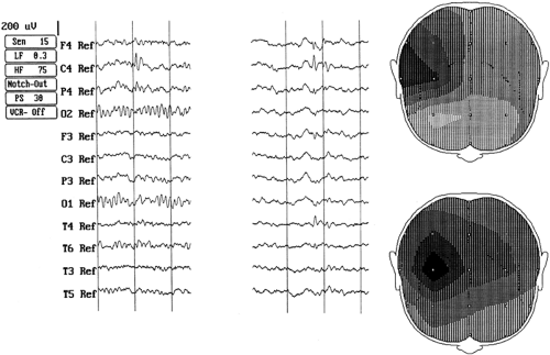 FIGURE 1. Examples of electroencephalogram s and maps of radial and tangential spikes. Tracing: left, radial; right, tangential; grid lines 1 second apart; ref, linked cheeks; negative up. Maps: top, tangential (T4-F4); bottom, radial (C4); nose-down vertex view; right, patient’s left. Color scale: white, positive; black, negative. |
Decomposition of Spikes
A segment of scalp EEG containing a single spike discharge might represent the aggregate of electrical activity from more than one source. In the presence of a high signal-to-noise ratio, as may be present with averaged spikes,24 it is possible to decompose this aggregate using mathematical techniques. The assumption is that such objective mathematical decomposition can represent separate physiologic sources, with no guarantee that such an interpretation is accurate or even appropriate. Nevertheless, the results can be useful in providing a measure of the electrical characteristics of the spike generators or sources. On this latter point, Wong84 reviewed the use of source behavior information in distinguishing populations of epileptic foci. FIGURE 2 is an example of an analysis using singular value decomposition (SVD).26 Principal component analysis can also be used to achieve substantially similar results, although SVD makes spatial displays more directly available.
From FIGURE 2, one can see that the original spike segment shows a complex topography over the right fronto-centrotemporal area, with the predominant negative spike peaking earliest at F4, then slightly later at C4, then still later at T4. Simultaneously with the F4 negative peak is a smaller, positive peak at T6. Under such careful scrutiny, there are, therefore, tangential and radial components within the single spike, lending to the suspicion that this was a complex spike, with perhaps complicated multiple generators. The decomposed features (1 and 3) provide mathematical (and objective) evidence of two separate sources, overlapping spatially but with distinct topography (tangential and radial). These two presumed separate sources might well originate from cortical areas with different clinical symptomatology.
Notwithstanding the cautionary note regarding the interpretation of each component as being from a separate source, such a hypothesis could be generated and tested against collected patient populations for verification, with particular emphasis on the clinical symptomatology and electroclinical correlations.
Kobayashi et al.33 reported being able to isolate separate epileptic components from spike and slow wave complexes using independent component analysis (ICA). They proposed that these components might represent separate cortical regions. Such a possibility would be of interest in the identification and surgical resection of the presumed neocortical focus. However, Unsworth et al.74 defined the criteria for the EEG data required for the ICA procedure to be reliable and interpretable. They concluded that it was not appropriate to apply ICA or source localization from independent components in four common types of childhood epilepsy. They also listed some preconditions before such analysis can be valid.
Related posts:

Stay updated, free articles. Join our Telegram channel

Full access? Get Clinical Tree


