Cytotoxic and transvascular oedema. (a) Normal—two astrocytes and a capillary. (b) Cytotoxic oedema: influxing water has caused the cells to swell, impinging on the extracellular space and leading to DWI signal changes on MRI. (c) Transvascular oedema—effluxing water from the capillary expands the extracellular space and leading to reduced density on CT
At this point, the intracellular space is overhydrated, but the extracellular space is dehydrated [20], usually resulting in no overall change to the water content of the brain tissue [18]. Cellular swelling impedes the diffusion of water in the extracellular space.
Late hyperacute (6–24 h): There is a variable degree of overlap with the early hyperacute phase, and cytotoxic edema may continue to progress as before. Cytotoxic edema enables transvascular edema to develop. Transvascular edema consists firstly of ionic edema, which is the passive diffusion of sodium and chloride ions, and subsequently water molecules, across the capillary membrane into the extracellular space [18]. As the blood–brain barrier degrades, intravascular proteins also pass into the extracellular space, drawing water by oncotic force, which is known as vasogenic edema [18]. The distinction between ionic and vasogenic edema may be theoretically important because blood–brain barrier breakdown may predispose to hemorrhagic transformation causing further deterioration in neurological function [21], but conventional neuroimaging is currently unable to distinguish the etiology of transvascular edema.
Transvascular edema is dependent upon some residual perfusion, so may affect the ischemic penumbra more than the core infarct [21].
By this point, both the intracellular and extracellular spaces are overhydrated, resulting in an increase in the water content of the brain tissue. Diffusion of water in the extracellular space is still restricted by cellular swelling.
Acute (1–7 days): There is considerable overlap between the late hyperacute and acute phases, but the distinction is important for stroke clinicians: patients presenting within the late hyperacute phase may still be eligible for time-dependent thrombolysis or thrombectomy treatment depending upon the residual ischemic penumbra, however once the acute phase has been reached these treatments may no longer be an option.
The water shift during this period is complex and not yet completely understood. Cytotoxic edema has usually peaked within the late hyperacute phase [19] and diminishes throughout the acute phase. Transvascular edema continues to progress, and the overall water content of brain tissue will peak between 2 and 4 days after stroke onset [22]. Despite the resulting reduction in the ratio of intracellular to extracellular space from 24 h onward, the restriction of water diffusion does not begin to relax until 5–7 days post onset [13] which suggests that cellular swelling due to cytotoxic edema cannot be the only cause for diffusion restriction. Alternative mechanisms for diffusion restriction in the acute phase may include a higher concentration of transvascular proteins and debris from apoptotic cells within the extracellular space.
Subacute (1–3 weeks): Many nonviable cells will have undergone apoptosis by the subacute phase. Transvascular edema will continue to resolve in the subacute phase but the extracellular space remains larger than in the pre-stroke brain, partly due to cellular necrosis, and partly due to expansion of the extracellular matrix from reactive astrocytes. The restriction of water diffusion will continue to relax, pseudo-normalizing at 10–15 days, before water diffusion increases above baseline levels due to the expanded extracellular space [16].
In the subacute phase, water in the extracellular space will begin to diffuse more freely even than in healthy brain tissue. The overall water content of the brain tissue remains high due to the expanded overhydrated extracellular space.
Chronic (>3 weeks): By this stage, edema has usually resolved. Parts of the brain tissue may form cystic areas full of CSF (cystic encephalomalacia). These areas are separated from surrounding healthy brain tissue by glial scars with an expanded extracellular matrix (gliosis).
Now that we have reviewed the pathophysiology of acute ischemic stroke, we can proceed to explore the individual neuroimaging methods and findings most commonly encountered in the emergency setting. We will do this by exploring a typical pathway through the different neuroimaging methods for a patient presenting with acute ischemic stroke, explaining how each method can impact upon the acute management of patients.
3 Neuroimaging Methods in Acute Stroke
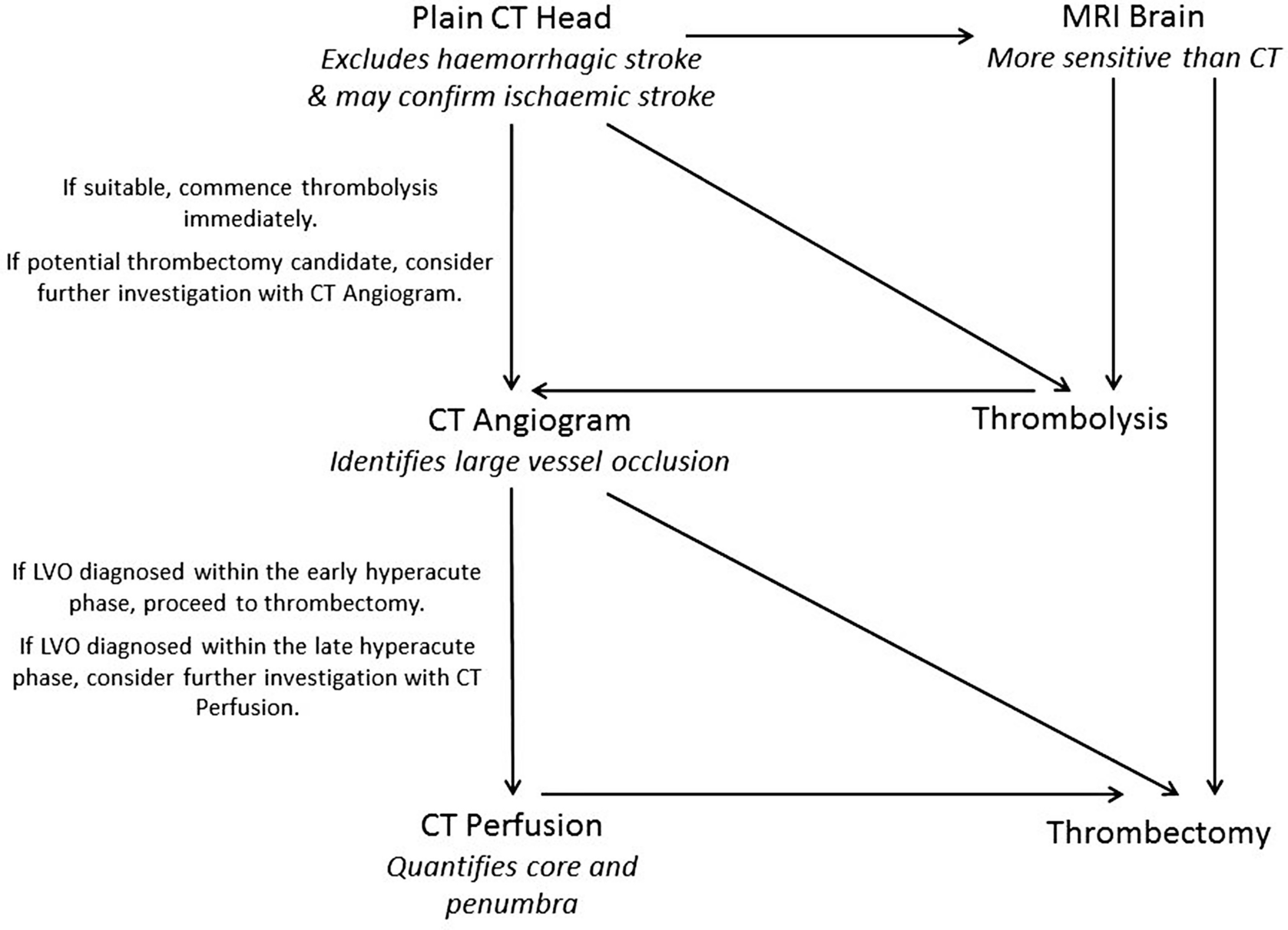
An example neuroimaging pathway for acute ischaemic stroke. Practice may vary from hospital to hospital. CT Angiogram and CT Perfusion may be replaced by MR Angiogram and MR Perfusion, depending upon local availability. If Perfusion imaging is not used then maximal standard timescales between stroke onset and thrombolysis is 4.5 h, and thrombectomy is 6 h
3.1 Plain Computed Tomography (CT)
3.1.1 Background
Computed Tomography (CT) is universally accepted as the best first choice neuroimaging investigation for acute stroke due to the short procedure time, availability and relatively easy interpretation. It is based upon the principle that physical density is proportional to attenuation of an X-ray beam. Complicated calculations are used to reconstruct a dataset from the X-ray detectors that describes the volume of the brain as a series of small cubes (voxels), each with a brightness that corresponds to the average density of the tissue within each voxel.
The CT scanner consists of a circle-shaped gantry with an X-ray tube source on one side and a detector array on the other side. The gantry rotates around the patient throughout the scan to acquire a series of projections across as many different angles as possible. Older scanners moved the table one step at a time, resulting in the acquisition of separate axial slices through the brain. This was a time-consuming process and resulted in a trade-off either between slices of the patient being skipped by the scanner, or multiple unnecessary irradiations of adjacent slices.
The newer generation CT scanners bypass this problem by utilizing multiple parallel arrays of detectors and continuously and simultaneously moving the table and rotating the gantry, resulting in the entire volume of the brain being scanned in a helical fashion. This has three advantages—first, the whole brain can now be scanned in a matter of seconds; second, the helix can be reconstructed into whatever spatial resolution (aka voxel size) is required, with an important caveat that we will address shortly; third, because the entire volume of the brain is imaged, images are no longer limited to the axial plane and can be reconstructed into sagittal and coronal views for ease of interpretation.
Plain CT is distinguished from other forms of CT by whether or not intravenous contrast is administered.
3.1.2 Advantages and Disadvantages
Advantages of plain CT are that it is relatively inexpensive, universally available including out-of-hours, easy to interpret, effective in ruling out hemorrhagic stroke, and there are no immediate safety exclusions.
The disadvantage for patients is that it involves exposure to ionizing radiation. For the clinician there is limited sensitivity in the hyperacute phase, limited distinction between large and small vessel occlusion and no information about core–penumbra mismatch.
3.1.3 Variable Parameters
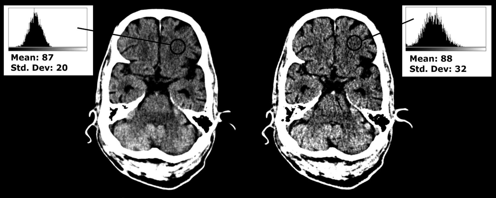
Thick and thin slices reconstructed from the same plain CT. Left: Thick (5 mm) axial slices demonstrate lower quantum noise, as evidence by a smaller standard deviation for a similar mean brightness (the numerical values of pixel brightness here do not reflect the true Hounsfield Unit values because these measurements were retrospectively obtained from JPEG images). Right: Thin (1 mm) axial slices provide a more accurate representation of hyperdense structures (the black arrow represents a hyperdense basilar artery in cross-section created because the lumen is full of fresh thrombus, not well visualised on the thick slice)
Thick slices result in a voxel size of around 1 mm (X) × 1 mm (Y) × 3–5 mm (Z). One advantage is that there are fewer images to store, transmit, and view. Furthermore, because more X-ray photons have contributed to the formation of each voxel in a thick rather than a thin slice, there is reduced quantum noise (which is the phenomenon that results in the black-and-white “grainy” random variation in CT images, similar to the static seen on analogue television sets). This makes thick slices the best choice to assess for parenchymal edema.
Thin slices result in a voxel size of around 1 mm (X) × 1 mm (Y) × 0.5–1 mm (Z). Their advantage is that they result in a more accurate representation of tissue density, because a shorter length of brain tissue is averaged to form each voxel. This makes thin slices the best choice for assessing for hyperdense tissue (such as arterial thrombus).
In-plane spatial resolution can also be improved by reducing the voxel size in the X and Y dimensions to <1mm, or by using a dedicated high resolution reconstruction filter known as a “bone”, “hard”, or “high resolution” kernel, but both options will increase the image noise. In situations where material contrast is naturally high and spatial resolution is critical (for example, investigation of potential skull fractures) it is better to use a high resolution kernel and smaller voxel size. Stroke patients sometimes present with a history of head trauma either preceding or following the onset of their stroke symptoms, and reconstruction of both high- and low-resolution kernel images may be performed for this reason. But low resolution or “soft” kernels should always be used to assess the brain parenchyma.
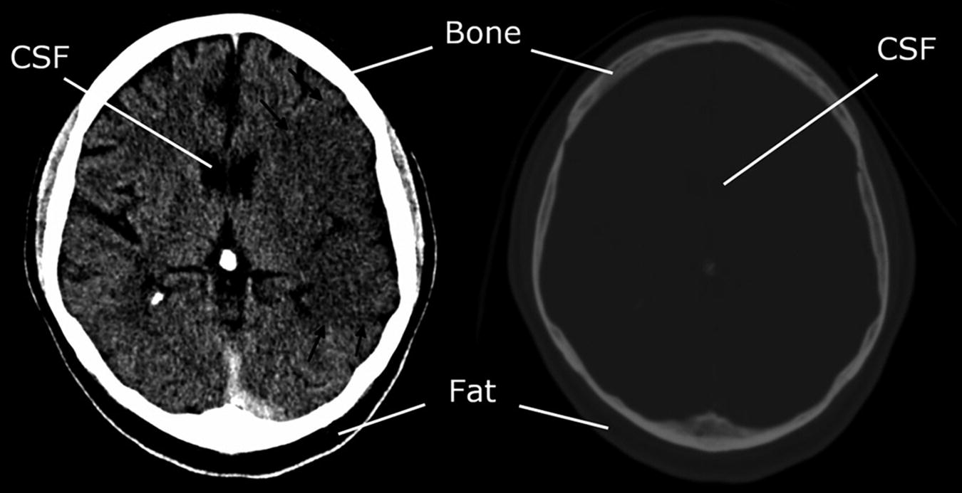
A demonstration of the power of windowing. Left: Narrow stroke windows (window width of 35 HU; window level of 40; range 5–75 HU). CSF and fat both appear black because they are below the range of the window. No internal bone structure is visualised because it is all above the range of the window. Right: Very wide windows (width 2000; level 1000; range: −1000 to 3000 HU). No tissue is either black or white because all tissues are within the window range. The relative differences between fat, CSF, white matter and grey matter are all insignificant compared to their difference from bone
3.1.4 Diagnostic Scope and Imaging Findings
Hemorrhagic Stroke
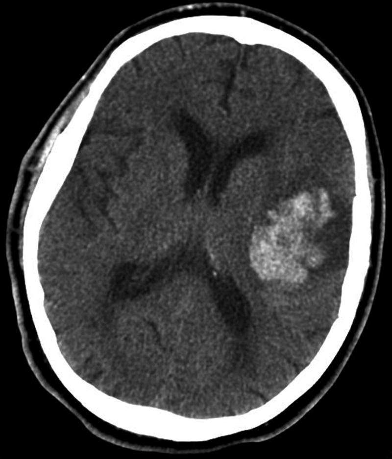
Plain CT showing acute intracerebral haemorrhage in the left cerebral hemisphere, which is easily identified by a markedly increased density within the brain parenchyma
Hyperacute Ischemic Stroke
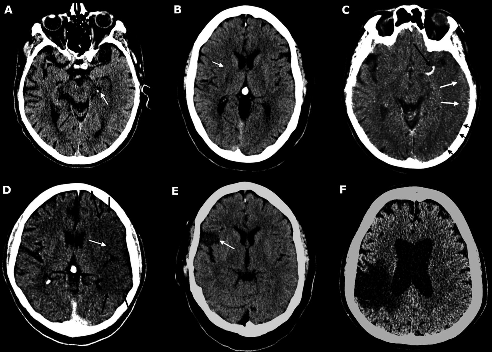
Plain CT findings throughout the evolution of ischaemic stroke. (a) Early hyperacute. Hyperdense left posterior cerebral artery (white arrow). No parenchymal changes. (b) Early to late hyperacute. Transvascular oedema results in the subtle loss of grey/white matter differentiation localised to the right putamen (white arrow), indicative of a right MCA stroke. No sulcal effacement. (c) Late hyperacute to acute. Left MCA contains hyperdense thrombus (long black arrow). Transvascular oedema results in poorly defined hypodensity within the left MCA territory with sulcal effacement (short black arrows). A small amount of grey matter can still be distinguished (white arrows). (d) Acute. Transvascular oedema results in a well-defined region of hypodensity within the left MCA territory (black arrows) with total loss of grey/white matter differentiation and sulcal effacement (white arrow). (e) Subacute. Necrosis and early gliosis evidence within a well-defined subset of the right MCA territory (white arrow). Internal contents are still denser than CSF (difficult to discriminate on such narrow stroke windows) indicating large amounts of cellular debris. Oedema within the neighbouring well perfused areas of the brain has resolved. (f) Chronic. Large region of brain affected by a stroke 20 years previously is very hypodense due to cystic encephalomalacia. The periphery of this region is chronically gliotic but this cannot be distinguished from cystic encephalomalacia on CT. We will distinguish the two later in this chapter using MRI images subsequently acquired from the same patient
The sensitivity of plain CT to diagnose ischemic stroke in the early hyperacute phase has been reported with a wide range in the literature [23], with one study suggesting it may be as low as 47% due to the limit in tissue density changes which can be detected by this single technology [25]. However, if clinicians are confident that their assessment of the patient makes stroke the likely diagnosis, a CT scan without hemorrhage or other pathological changes will be judged as consistent with a clinical impression of ischemic stroke and used to support a tPA or anticoagulation treatment decision. It is not necessary to show evidence of thrombus to initiate tPA as many smaller lesions cannot be identified, but there is still an advantage from treatment.
Late Hyperacute or Acute Ischemic Stroke
Unlike MRI, plain CT is unable to image the compartmental redistribution of water within the brain parenchyma. However, it is able to image changes in the average water content of brain tissue across both intracellular and extracellular compartments, and the increased water content in acute stroke will result in a lower density of the brain parenchyma. This is most easily identified by a region of hypoattenuation within the brain parenchyma, usually visible only once the stroke has passed the early hyperacute phase into the late hyperacute or early acute phases. Later acute or subacute changes include a discernible increased volume of brain parenchyma, evidenced by effacement of the cerebral sulci (Fig. 6d). Consequently, the sensitivity of CT performed within 7 days of onset is greater than in the early hyperacute phase alone [23] and has been reported between 63–95% [26–28].
3.1.5 Quantitative Plain CT
Plain CT interpretation, like most neuroimaging methods, is normally achieved qualitatively in clinical practice. However, the Alberta Stroke Program Early Computed Tomography Score (ASPECTS) is often used as a quantitative plain CT score. It is a ten-point scale which divides the brain supplied by the anterior circulation into anatomical segments and deducts a point for each region that has infarcted or shows early ischemic changes [29]. A detailed explanation of the score and training to apply it is available at www.aspectsinstroke.com. ASPECTS is gaining favor as an approximate surrogate biomarker for core infarct volume, with one study finding that an ASPECTS of <7 can predict an infarct core of 70 mL or larger on diffusion MRI with 74% sensitivity and 86% specificity [30]. ASPECTS has been used in the patient selection process for large thrombectomy trials in the early exclusion of patients with large established infarct cores without the need for advanced imaging [31, 32], and its role in thrombectomy selection has been acknowledged by the international stroke community [33, 34].
3.1.6 Impact of Plain CT upon the Acute Stroke Treatment Pathway
Plain CT remains the first line neuroimaging method in the setting of acute stroke because it is effective at filtering out patients with hemorrhagic stroke [23], enabling early administration of thrombolytic agents. It can also provide a crude way of separating chronic from acute stroke; however, it is limited in its ability to identify patients suitable for treatment with thrombectomy: patients who are still potentially eligible for treatment with thrombectomy following a plain CT should undergo further investigation with CT Angiography.
3.2 CT Angiography
3.2.1 Background
CT Angiography (CTA) fundamentally differs from plain CT in its use of intravenous contrast agent administration. Iodine is favored almost universally because it is relatively biologically inert, yet physically much denser than soft tissue. A good quality intracranial angiogram will increase the density of the arteries ideally above 250 HU, almost an order of magnitude higher than the density of the brain parenchyma. The increase in the density of opacified arteries relative to the brain parenchyma results in the ability to directly visualize the patency of the intracranial arteries and those in the neck. It is increasingly being performed routinely during the assessment of patients arriving in hospital within a timescale that may be suitable for thrombectomy, which requires direct visualization of a potentially accessible thrombus before removal is attempted.
3.2.2 Advantages and Disadvantages
The advantages of CTA are its ability to distinguish large from small vessel occlusion, localize the thrombus within the arterial tree, and visualize the collateral circulation to the region of stroke. It is readily available quickly and out-of-hours within clinical services.
The disadvantages for patients are an exposure to ionizing radiation and the use of intravenous contrast medium which carries a risk of renal injury. For clinicians there is limited use in assessing the core–penumbra mismatch and it is not suitable for assessing brain parenchyma.
3.2.3 Variable Parameters (Further to Those Described for Plain CT)
The field-of-view for CTA depends upon the purpose of the imaging. When investigating for intracranial arterial aneurysms, only the brain (from the circle of Willis to the cranial vertex) needs to be imaged, whereas identification of carotid stenosis (e.g., as part of the workup for treatment of a transient ischemic attack) requires only the carotid arteries to be imaged. If investigating for large vessel occlusion, both the carotid arteries and the intracranial arteries need to be imaged. This field-of-view is sometimes described as arch to vertex.
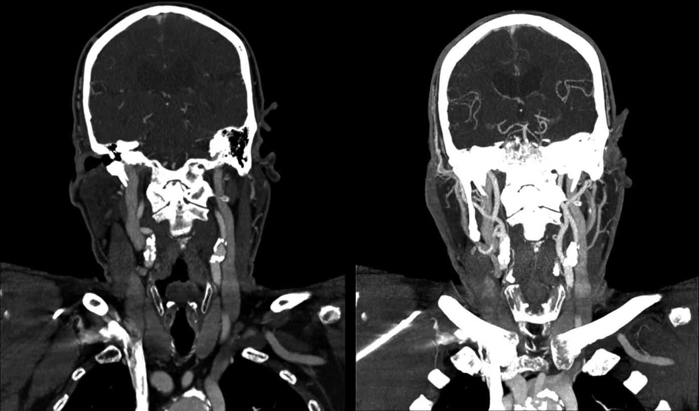
Standard coronal thick slices compared to MIPs from a CT Angiogram. Left: 5 mm coronal thick slices. The intracranial arteries are moving in and out of plane, therefore appear fragmented and it is necessary to look at multiple slices or a computer constructed 3D view. Right: 20 mm coronal MIP formed from four adjacent 5 mm slices. The path of the artery from each constituent slice is mapped on the MIP image enabling the arterial tree to be followed with greater ease
The Contrast Phase refers to the time delay between injecting the contrast and performing the scan. The contrast bolus has to travel from a cannulated peripheral vein, through the right heart, into the lungs, into the left heart and through the aortic arch before it can reach the carotid and vertebral arteries that ultimately supply the brain. Historically CTAs were performed by scanning with a fixed delay of around 20 s after bolus injection so that the contrast medium had time to reach the cerebral circulation, however due to heterogeneity in the length of time taken for the bolus to travel from vein to brain, suboptimal opacification of the intracranial arteries used to be a frequent problem. Modern scanners use bolus tracking technology to overcome this. More recently, the technique of multiphase CTA has been developed. This involves rescanning the brain after a normal bolus-tracked arch to vertex CTA, usually an additional two times, with all acquisitions separated by around 8 s [35]. This enables the temporal resolution of arterial blood flow, which can overcome the shortcomings of conventional CTA in assessing the collateral circulation [35, 36].
3.2.4 Diagnostic Scope and Imaging Findings
Identifying Large Vessel Occlusion (LVO)
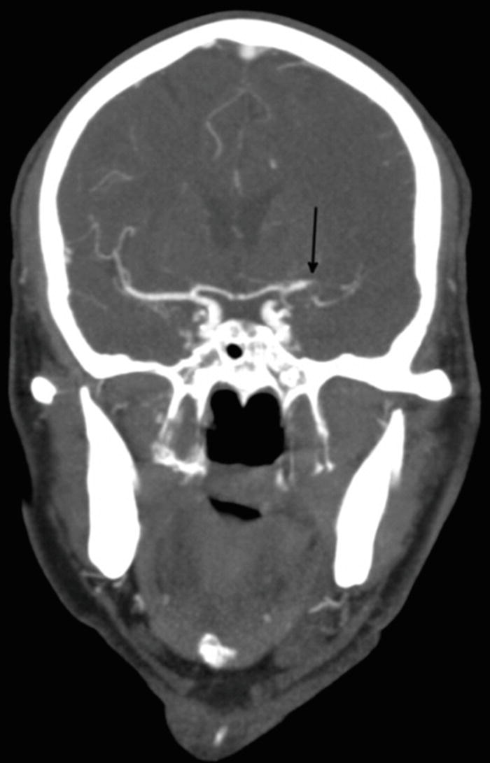
Five millimeter coronal slice from an abnormal CTA demonstrates an occlusion of the left MCA (black arrow). This is an anterior proximal large vessel occlusion that may be treatable with thrombectomy
Neurointervention Planning
Aside from its use in treatment decisions and stratification of patients, knowing the location of the LVO can help neurointerventionists plan their intervention (e.g., where they should expect to place the arterial catheter device). Similarly, the assessment of the common and cervical internal carotid arteries is invaluable to the neurointerventionist: sometimes patients can present with tandem occlusion, consisting of an intracranial LVO in addition to extracranial internal carotid arterial obstruction, and these patients may require additional management such as carotid stenting prior to accessing the intracranial circulation [42].
Assessing the Collateral Circulation
Collateral scoring using multiphase CTA has been used successfully to identify patients with different outcomes in the process of selection for thrombectomy in one clinical trial. Patients with a “better” score had a better outcome, reflecting the increased blood flow to the penumbra from the additional collateral vessels [31]. Multiphase CTA provides an attractive compromise between providing information that can help select the ideal candidates for thrombectomy, but with relatively little modification to conventional CTA protocols: it could therefore be adopted relatively easily by all departments currently offering single phase CTA. Despite the promising early results and potential transferability of this neuroimaging method, it is still in its relative infancy and further validation from future studies would be useful.
3.2.5 Impact of CTA upon Acute Stroke Management Pathway
The optimum neuroimaging methods for patient selection for thrombectomy have not yet been established, and the decision to treat is still made on a case-by-case basis following urgent multidisciplinary discussion involving a neurointerventionist and a stroke physician [33]. The importance of CTA in making these decisions cannot be underplayed, as the only other noninvasive neuroimaging method that can diagnose and localize LVO effectively is magnetic resonance angiography (which is more expensive and far less available than CTA). For patients presenting in the early hyperacute phase with a proximal large vessel occlusion on CTA and evidence of a small infarct core on plain CT, the decision to proceed to thrombectomy can sometimes be made at this stage with no further neuroimaging until the procedure itself [33]. Sometimes the decision to treat is more complicated, for example if patients present in the late hyperacute phase: some of these patients may benefit from thrombectomy up to 24 h post-onset, dependent upon the collateral circulation, volume of salvageable tissue and size of the core infarct [15]. The distinction between infarct core and ischemic penumbra can be investigated further with CT Perfusion.
3.3 CT Perfusion
3.3.1 Background
CT Perfusion (CTP) is typically used to determine how much of the brain tissue is viable: typically, ischemic strokes will consist of a central infarct core which cannot be salvaged, surrounded by an ischemic penumbra which may be salvaged by reperfusion therapy. Other methods of neuroimaging are able to quantify the infarct core volume alone (ASPECTS or diffusion MRI), but perfusion imaging is able to quantify both the infarct core and, uniquely, the ischemic penumbra by directly imaging cerebral blood flow.
Mean transit time (MTT), which reflects the length of time that a red blood cell spends within a given volume of brain tissue (unit: s).
Cerebral blood volume (CBV), which reflects the total volume of blood within the tissue, per unit mass of brain tissue (unit: mL/100 g).
Cerebral blood flow (CBF), which reflects the rate at which the tissue fills with blood, per unit mass of brain tissue (unit: mL/s/100 g).
Stay updated, free articles. Join our Telegram channel

Full access? Get Clinical Tree


