(1)
for 1 ≤ i ≤ N, where v i denotes the membrane voltage of neuron i, μ is a dc component in the noisy synaptic input and τ is the membrane time constant for the subthreshold dynamics. We adopt the standard threshold-spike-reset condition [8]: a spike is emitted whenever v i (t) = V T , and after that the voltage is reset and held at v i (t +) = V R during a refractory period τ R . Additionally, s(t) is a common component in the input and the Gaussian white noise η i (t) (1 ≤ i, j ≤ N) models the internal stochastic component for the ith neuron. For each neuron, the output spike train y i (t) = ∑ k s(t − t i k ) with t i k being the kth spike time is of interest, and the average spike train
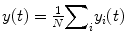 is taken as the output for summing parallel array. We assume that for 1 ≤ i, j ≤ N there is
![$$ \left\langle {\eta}_i(t){\eta}_j\left(t+\tau \right)\right\rangle =\left[{\delta}_{i,j}+c{\delta}_{i,i+1}\right]\delta \left(\tau \right) $$](/wp-content/uploads/2016/09/A315578_1_En_30_Chapter_Equ2.gif)
(2)
Since the local spatial correlation does not affect the response of each neuron, it is necessary to obtain the spectral statistics 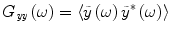 for the ensemble output spike train, where
 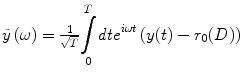 is the Fourier transform of the zero average output spike train with r 0(D) being the stationary firing rate at the noise level D. For this aim, let us resort to technique of linear approximation [9–11]. According to linear approximation, each neuron can be regarded as a linear filter, and thus the frequency domain linear response for each neuron can be approximated as
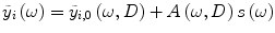
where  is the unperturbed part of stationary spectral density
 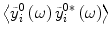 and A(ω, D) is linear susceptibility on the noise level of D. The stationary spectral density [12] and the linear susceptibility [13, 14] are explicitly given as
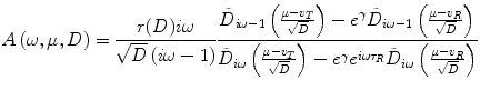
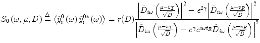
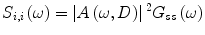
with ![$$ \gamma =\left[{v}_R^2-{v}_T^2+2\overline{\mu}\left({v}_T-{v}_R\right)\right]/4D $$](/wp-content/uploads/2016/09/A315578_1_En_30_Chapter_IEq6.gif) . And then from Eq. (3), the auto-spectral density
. And then from Eq. (3), the auto-spectral density 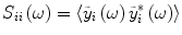 for the ith neuron is obtained as
 Integrated Neuropsychiatric Assessment System: A Generic Platform for Cognitive Neurodynamics Research
 Dynamic Temporal-Topological Structure of Brain Network Within ADHD
 Activity Patterns in Cortical Dynamics and the Illusion of Localized Representations
 on the Neural Energy Coding
 Cortical Singularities During the Cognitive Cycle Using Random Graph Theory
 as Bifurcations Shaped Through Sequential Learning


for the ensemble output spike train, where is the Fourier transform of the zero average output spike train with r 0(D) being the stationary firing rate at the noise level D. For this aim, let us resort to technique of linear approximation [9–11]. According to linear approximation, each neuron can be regarded as a linear filter, and thus the frequency domain linear response for each neuron can be approximated as(3)
is the unperturbed part of stationary spectral density and A(ω, D) is linear susceptibility on the noise level of D. The stationary spectral density [12] and the linear susceptibility [13, 14] are explicitly given as(4)
(5)
. And then from Eq. (3), the auto-spectral density for the ith neuron is obtained asRelated posts:
Integrated Neuropsychiatric Assessment System: A Generic Platform for Cognitive Neurodynamics Research
Dynamic Temporal-Topological Structure of Brain Network Within ADHD
Activity Patterns in Cortical Dynamics and the Illusion of Localized Representations
on the Neural Energy Coding
Stay updated, free articles. Join our Telegram channel
Full access? Get Clinical Tree
