Physiologic Basis of the Electroencephalogram and Local Field Potentials

György Buzsáki

Roger D. Traub

Introduction

Analyses of electric and magnetic fields and imaging energy production in brain structures are the principal instruments in the arsenal of contemporary neuroscience for noninvasive studies of the brain. Three fundamental methods can provide high temporal resolution of neuronal interactions at the network level—electroencephalogram (EEG), magnetoencephalogram (MEG),³¹ and, in invasive experiments, voltage-sensitive, dye-based optical imaging²⁸ (see Chapters 74, 75, 76, 77, 80, 87, and 90). Each of these methods has its advantages and shortcomings. A common major obstacle of clinical EEG, MEG, and optical imaging methods is that their “views” are confined mostly to surface events (although MEG, in principle, can provide information about depth events as well⁶²^,⁶³). However, most network interactions occur in the depth of the cortex. Although imaging methods provide significant spatial resolution, including deep structures in the brain, all of these “global” methods face the same fundamental question—the “reverse engineering” problem of signal interpretation.⁶² The signals measured by EEG and MEG reflect the cooperative actions of neurons. Therefore, full understanding of the signals recorded by these methods is possible only after their cellular-synaptic generation is explored. Nevertheless, even without a full deciphering of the origin of the recorded signal, EEG and MEG provide useful information about brain operations in health and disease, and EEG evaluation remains the essential method for the diagnosis of epilepsy.

Membrane currents generated by neurons pass through the extracellular space. These currents can be measured by electrodes placed outside the neurons. The field potential (i.e., local mean field) recorded at any given site reflects the linear sum of numerous overlapping fields generated by current sources and sinks distributed along multiple cells. This macroscopic state variable is referred to as local field potential (LFP) if measured by a small electrode in the brain, an electrocorticogram (EcoG) if measured by, for example, subdural grid electrodes, and EEG if recorded from the scalp, or an MEG as monitored with magnetosensor semiconductor quantum interference devices (SQUIDs). LFPs provide experimental access to the spatiotemporal activity of afferent, associational, and local operations in a given structure. Field potential measurements provide the best experimental and clinical tools for assessing cooperative neuronal activity at high temporal resolution. However, without a mechanistic description of the underlying neuronal processes, the mean fields recorded by these methods are a gross correlate of brain activity rather than a predictive descriptor of the specific functional/anatomic events.

Scalp recordings offer only limited information about the structures and neuron groups from which the electrical activity emanates, and the inverse problem does not have a unique solution. The difficulty of source localization using scalp EEG has to do with the low resistivity of neuronal tissue to electrical current flow, the capacitive currents produced by the lipid membranes, and the distorting and attenuating effects of glia, blood vessels, pia, dura, skull, scalp muscles, and the skin. As a result, the EEG recorded by a single electrode becomes a spatially smoothed version of the local field potentials under a scalp surface on the order of 10 cm², and under most conditions has little discernible relationship with the specific patterns of activity of the neurons that generate it.⁶² The spatial resolution can be improved with intracranial electrodes such as subdural grid electrodes. Nevertheless, because current density, that is, the spatial derivative of current, is sensitive mainly to superficial sources, the signals recorded by scalp or grid electrodes sample mostly the electrical activity that occurs in the superficial layers of the cortex. The contribution of deeper layers is scaled down substantially, whereas the contribution of neuronal activity from below the cortex is, in most cases, virtually negligible. This “fish-eye lens” scaling feature of EEG is the major theoretical limitation for improving its spatial resolution.

A straightforward approach to deconvolving the surface-recorded event is simultaneously to study electrical activity on the surface and at the sites of the extracellular current generation in experimental situations. LFP measurements (sometimes referred to as “micro-EEG”⁶⁸) combined with recording of neuronal discharges is the best experimental tool available for studying the influence of cytoarchitectural properties, such as cortical lamination, distribution, size, and network connectivity of neural elements, on electrogenesis. However, large numbers of observation points combined with decreased distance between the recording sites are required for high spatial resolution and for making interpretation of the underlying cellular events possible. Progress in this field has been accelerated by the availability of micro-machined silicon-based probes with numerous recording sites.¹²^,⁹² The information obtained from the depth of the brain can then assist with the interpretation of the surface-recorded events.

In principle, every event associated with membrane potential changes of individual cells (neurons, glia) contributes to the perpetual voltage variability of the extracellular space. Until recently, synaptic activity has been viewed as the exclusive source of extracellular current flow or EEG. As will be discussed, however, synaptic activity is only one of the several membrane voltage changes that contribute to the measured field potential. Progress during the last decade has revealed numerous sources of relatively slow membrane potential fluctuations not directly associated with synaptic activity. Such nonsynaptic events also may contribute significantly to the generation of local field potentials. Accordingly, this chapter focuses on the cellular origin
of the extracellular fields. The reviews by Hämäläinen et al.³¹ and Okada et al.⁶⁴ provide detailed theoretical background for MEG and SQUIDs and compare EEG and MEG signal detection problems.

Measuring extracellular current flow: A TUTORIAL

Although a variety of sources can contribute to the extracellular current flow (see later discussion), for simplicity, we consider only synapse-mediated events in this section. For the transmembrane potential to change in a given neuron, there must be a transmembrane current, that is, a flow of ions across the membrane. This is the event that one has to spatially localize for the interpretation of the extracellular current or voltage. Opening of membrane channels (or more precisely, an increase in their open-state probability) allows transmembrane ion movement, that is, current flow. LFP (i.e., local mean field) recorded at any given observation point reflects the linear sum of numerous overlapping fields generated by current sources (e.g., current from the intracellular space to the extracellular space) and sinks (current from the extracellular space to the intracellular space) distributed along multiple neurons.

The term “field” is often used differently by electrophysiologists and physicists. For the physiologist the field or local field typically means extracellular potential, whereas in physics the gradient of the field is referred to as electric potential. The field is defined at every point of space from which one can derive the force “felt” by an electric charge at that point. The field can be transmitted through volume and is known as volume-conduction. Lower-frequency currents produce, or correspond to, transmembrane currents over larger spatial extent of membrane than are fast signals, partially because the space constant of the dendritic cable is shorter for high frequencies than low frequencies. Furthermore, because the lipid membrane of neurons, glia, and other cells in the brain acts as a capacitive low-pass filter, it offers an easier passage to low-frequency signals than to high-frequency signals. As a result, slow signals, such as postsynaptic potentials, can propagate much farther in the extracellular space than can spikes. In addition, longer-duration events (e.g., excitatory and inhibitory postsynaptic potentials [EPSPs and IPSPs]) have a much higher chance of occurring in a temporally overlapping manner than do the very brief action potentials. Finally, many more neurons display EPSPs and IPSPs than fast spikes in a given temporal window because only a very small minority reaches the spike threshold at any instant in time. For these reasons, the contribution of action potentials to the LFP and especially to the subdural ECoG or scalp EEG in the normal brain is practically negligible. This is not necessarily the case under epileptic conditions, however, when neurons can synchronize within the duration of action potentials. The synchronously discharging neurons create local fields, known as compound or “population” spikes.

Excitatory currents, involving sodium (Na⁺) or calcium (Ca²⁺) ions, flow inwardly at an excitatory synapse (i.e., from the activated postsynaptic site to the other parts of the cell) and outwardly away from it. The passive outward current far from the synapse is referred to as a return current from the intracellular milieu to the extracellular space. Inhibitory loop currents, involving chloride (Cl^–) or potassium (K⁺) ions, flow in the opposite direction. Viewed from the perspective of the extracellular space, membrane areas where current flows into or out of the cells are termed sinks or sources, respectively. The current flowing across the external resistance of the extraneuronal space sums with the loop currents of neighboring neurons to constitute the local mean field or LFP. In short, extracellular fields arise because the slow EPSPs, IPSPs, voltage-gated active currents, and other intracellular events (see later discussion) allow for the temporal summation of currents of relatively synchronously activated neurons.

Depending on the size and placement of the extracellular electrode, the volume of neurons that contributes to the measured signal varies substantially. With very fine electrodes, LFPs reflect the synaptic activity of tens to perhaps thousands of nearby neurons only. LFPs are, therefore, the electric fields that reflect a weighted average of input signals on the dendrites and cell bodies of neurons in the vicinity of the electrode. If the electrode is small enough and placed close to the cell bodies of neurons, extracellular spikes can also be recorded. Not surprisingly, in such a small volume of neuronal tissue, one often finds a statistical relationship between local field potentials, reflecting mostly input signals (EPSPs and IPSPs), and the spike outputs of neurons.⁴² The reliability of such relationship, however, progressively decreases with increasing electrode size, by lumping together electric fields from increasingly larger numbers of neurons. This is why the ECoG or scalp EEG, the spatially smoothed version of the LFP at numerous contiguous sites in a volume, often has a poor relationship to the spiking activity of individual neurons.

In deciphering the current source–sink origin of the local fields, we have to go “backward” from LFP measurement to cellular-synaptic current sources.⁵⁷ Current density is the current entering a volume of extracellular space. The current flow between two recording sites can be calculated from the voltage difference and resistivity using Ohm’s law, provided that information about the conductance (inversely proportional to resistivity) of the tissue is available. The conductance is a factor of both conductivity and the specific geometry of volume. If at least three linearly spaced electrodes are placed in the brain tissue, one can measure the voltage between the middle electrode and the two side electrodes and calculate the current flow between the pairwise sites. The difference between the respective current flows (i.e., the change over distance) is proportional to current density. More precisely, the current density is a vector reflecting the rate of current flow in a given direction through the unit surface or volume (measured in amperes/m² for a surface and amperes/m³ for a volume).²⁵^,⁵⁶^,⁶⁰

To illustrate the utility of the foregoing approach, consider a distant current source relative to the three equally spaced recording sites (Fig. 1). Each electrode will measure some contribution of the field (due to the passive return currents that pass through the extracellular space) from the distant source. Because the source is outside of the area covered by the electrodes, the voltage difference will be the same between the middle and side electrodes. Taking the difference between the voltage differences (voltage gradient), we get a value of zero, an indication that the measured field did not arise from local activity but was volume-conducted from elsewhere. In contrast, if the three electrodes span current-generating neuron groups, the voltage gradients will be unequal and their difference will be large, indicating the local origin of the current. By placing more microelectrodes closer to each other, one can more precisely determine the maximum current source density (CSD) and, therefore, the exact location of the maximum current flow.

Unfortunately, from CSD measurement alone, one cannot conclude whether, for example, an outward current close to the cell body layer is due to active inhibitory synaptic currents or reflects the passive return loop current of active excitatory currents produced in the dendrites. Without additional information that can clarify the nature of the current flow, the anatomic origin is ambiguous. The missing information can be obtained by simultaneous intracellular recording from representative neurons that are part of the population responsible for the generation of the local current. Alternatively, one can record extracellularly from identified pyramidal cells and interneurons and use the indirect spike-field correlations to determine whether, for example, a local current is an active,
hyperpolarizing current or a passive, return current from a more distant depolarizing event. Only after taking these extra steps one can pin down the current sources and sinks and make hypotheses about their synaptic-cellular origin. The combined information is very useful because it provides clues about the synaptic inputs to the same set of neurons whose outputs (i.e., spiking) can also be simultaneously monitored, provided that the recording electrodes are small enough. Once we have information about both the input and output of a small collection of neurons working together, we can begin to understand the transformation rules governing their cooperative action. This approach is the next best thing to the ideal condition when all inputs (synapses) and outputs of each cell are monitored simultaneously and continuously.

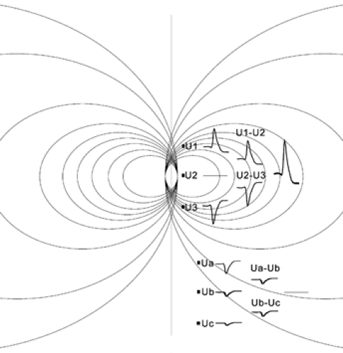FIGURE 1. Identifying current sources. Current source–sink dipole imbedded in a homogeneous and isotropic conductive medium. The density of lines reflects density of currents. The potential generated by the active dipole decays in the medium as the inverse square of the distance (not properly shown proportionally here, for illustrative purposes). The potentials measured at equally spaced locations, relative to an ideal infinite site (reference), are shown as U1, U2, and U3 close to the dipole, and Ua, Ub, and Uc far from the dipole. The differences of the potentials are shown in the middle row and the difference of the differences on the right. In a nonhomogeneous, nonisotropic medium, such as the brain, the current is flow is calculated as the ratio between the voltage (difference) and tissue conductivity (according to Ohm’s law). Although dipole-induced voltages can be measured far from the source, calculation of current density by three simultaneously recorded sites is spatially confined and can help to identify the anatomic location of the dipole.

Figure 2 illustrates the necessary steps in the identification of network mechanisms of evoked and spontaneous field events. The example is taken from the hippocampus because it is a simple, three-layered structure consisting of orderly arranged principal cells (pyramidal and granule cells) and interneurons. Therefore, the synaptic interpretation of the extracellular current is simpler than in multilayered structures. Activation of the excitatory associational input by electrical stimulation will depolarize the mid-apical and basal dendrites of pyramidal cells (shown in blue in FIGURE 2). The passive return current will flow out of the cells at the level of the neuronal bodies and distal apical dendrites (shown in red in FIGURE 2) specify where exactly (Figure D or 2E). This change in voltage is reflected by the characteristic depth distribution of field potentials. The extracellular voltage is negative close to the excitatory synapse and positive in the cell body layer. The reason for this is the large depolarization of the dendrite and the gradual decrease of intracellular depolarization toward the soma. This synaptic activity–induced intracellular voltage difference between the dendrites and soma (a “dipole”) will result in a current flow across the resistive membrane (arrows in FIGURE 2F). Simultaneous events in many neighboring pyramidal cells will linearly sum and produce an extracellular voltage fluctuation that can be measured with closely spaced electrodes. After determining the resistivity (impedance in case of an alternating current signal) characteristics of the extracellular space, we can calculate the local currents and current densities from the voltage measurements.²⁵^,⁶⁰

Increased afferent discharge also activates interneurons, some of which terminate on the cell bodies of the pyramidal cells. For example, the discharging basket cells release gamma-aminobutyric acid (GABA) and activate Cl^– channels, which allows the entrance of the negatively charged ion with resulting hyperpolarization of the pyramidal cell somata. Somatic hyperpolarization, in turn, creates a voltage gradient between the soma and dendrites (inhibitory dipole). The created intracellular voltage difference is the driving force of charges across the cell membrane and the consequent spatially distributed current flow in the surrounding extracellular fluid (FIGURE 2). Note that the direction of current flow is the same as in the case in which the driving force is apical dendritic depolarization (active sink). Because the direction of current flow is identical for dendritic excitation and somatic inhibition, the excitatory and inhibitory currents will sum in the extracellular space, resulting in large-amplitude field potentials. Because the excitation-concurrent somatic inhibition may prevent the depolarization of the axon initial segment and, consequently, the occurrence of action potentials, large-amplitude extracellular current flow can be associated with no spike output from pyramidal neurons. Thus, the relationship between dendritic excitation and spike output of pyramidal cells is highly nonlinear, and is largely determined by the state of inhibition.

Provided that dendritic excitation is strong enough to override somatic inhibition, the cells may discharge. In the simplest case, a Na⁺ spike will be generated in the initial segment of several neighboring pyramidal neurons. The large inward current associated with the spikes is reflected by a negative change of the extracellular voltage at the level of the axon initial segment/cell body accompanied by a smaller-amplitude, extracellular positive deflection out in the dendritic regions for the same reasons as described previously for the EPSPs. However, because the spatial location of this event is opposite to the afferent excitation of dendrites, the direction of the extracellular current flow will also be opposite. The contribution of fast spikes to the extracellular mean field is due to the hypersynchronous discharge of many pyramidal neurons (population spike) as a result of artificial stimulation of an afferent bundle. Interpretation of the extracellular events after the population spike is not straightforward, however, due to complex feedback effects of the network and other nonsynaptic events (see later discussion).

Once a circuit, such as that shown in FIGURE 2, has been “calibrated” by electrically evoked potentials, one can move to the next step—network-level description of the generation of spontaneous EEG events. The tutorial example we use is an intermittently occurring, large-amplitude hippocampal sharp wave (SPW). SPWs are present during immobility, consummatory behaviors, and slow-wave sleep. It is important that the events to be analyzed are clearly separable from other waveforms. After extracting the invariable features of this EEG pattern by averaging or other pattern recognition methods, we convert the

simultaneous voltage measurements into a CSD map (Figures 2D and 2E). Note that the distribution of the sinks and sources of SPWs is strikingly similar to the potentials elicited by stimulation of the associational/commissural inputs to the pyramidal cells. Comparison of the spontaneous and evoked events, therefore, allows the conclusion that activation of the same afferent pathways and neurons brings about both events. Indeed, independent experimental work revealed that SPWs in the hippocampus arise from the quasi-synchronous discharge of CA3 pyramidal neurons, the source of associational and commissural afferents to the CA1 region.¹¹^,¹⁶ Temporally overlapping activation of converging activity on single CA1 pyramidal cells results in a large depolarization of the dendrites, similar to the depolarization of these cells when the associational pathways are electrically activated. These extra- and intracellular events therefore provide circumstantial evidence that the same neuronal machinery is activated during spontaneously occurring SPWs as during electrical stimulation of the associational afferents.

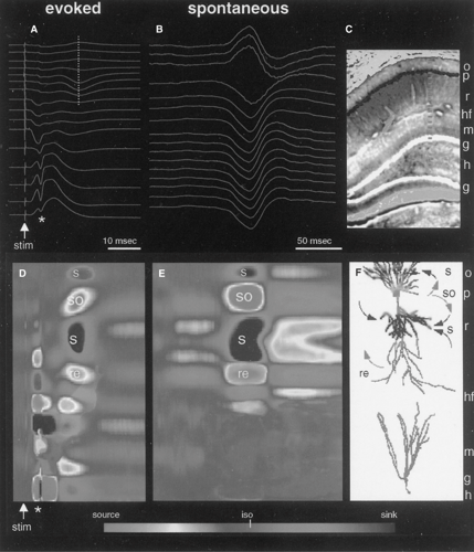FIGURE 2. Generation of extracellular field potentials. A: Simultaneously recorded evoked field responses in the CA1-dentate gyrus axis of the rat hippocampus in response to stimulation of the entorhinal input (stim). The asterisk indicates the population discharge of the monosynaptically activated granule cells. Their discharge, in turn, activates CA3 pyramidal cells (not shown), whose associational collaterals depolarize CA1 pyramidal cells and interneurons. This trisynaptic activation of CA1 pyramidal cells is reflected as a late field event (vertical dotted line). B: Spontaneously occurring sharp wave recorded during immobility. The traces are averages of 40 individual events. C: A frontal section of the hippocampus indicating the contact sites of the recording silicon probe (small squares). o, stratum oriens; p, pyramidal layer; r, stratum radiatum; hf, hippocampal fissure; g, granule cell layer; h, hilar region. D, E: Current-source density (CSD) maps of evoked field responses to perforant path stimulation (D) and of the spontaneous SPW pattern. Sinks (s, inward currents) and sources (so, outward currents) are indicated by cold and warm colors, respectively. iso, zero-current flow. The time scales in panels A and D, and B and E, are the same. F: Interpretation of the current sinks and sources on the basis of anatomic connectivity. Recorded layers are shown on the right of the pyramidal cell (above) and granule cell (below). Putative active currents are indicated on the right, and passive return (re) currents on the left of the pyramidal neuron. Note identical current sink–source distribution of the evoked and spontaneous events in the CA1 region (compare panels D and E). Sinks in stratum radiatum and oriens reflect excitation of the apical and basal dendrites of CA1 pyramidal cells, respectively, by the associational (Schaffer) collaterals of the CA3 region. The large source in the pyramidal layer is a combination of active outward current due to hyperpolarization of the soma by the simultaneously activated basket cells (not shown) and passive return currents from the sinks generated in the basal and apical dendrites. The source in the distal apical dendrites (re) is assumed to represent a passive return current due to the active sink in the middle of stratum radiatum. In addition to excitatory postsynaptic potentials, dendritic Ca²⁺ spikes may also contribute to the sinks in strata oriens and radiatum (see FIGURE 4). (From Buzsáki G, Traub RD. Generation of EEG. In: Engel J Jr, Pedley TA, eds. Epilepsy: A Comprehensive Textbook. Lippincott-Raven Press; 1996, with permission).

The contribution of GABA_a receptor–mediated inhibitory currents is generally believed to be small, based on the assumption that because the Cl^– equilibrium potential is close to the resting membrane potential, the change of the transmembrane voltage is limited. However, in actively spiking neurons, when the cell body is depolarized, the transmembrane potential mediated by GABA_a receptors can be large. Another cautionary note is that inhibition operates also on the dendrites, causing current flow opposite to the direction of excitatory currents. For the identification of excitatory and inhibitory components, represented by the extracellular current flow, a precise knowledge of the anatomic network is essential. Detailed physiologic experiments, including recordings from anatomically identified interneurons and pyramidal cells as well as differential pharmacologic blockage of the excitatory and inhibitory synapses, can provide further knowledge necessary for the proper interpretation of the observed sinks and sources (Fig. 3).⁴³^,⁴⁴^,⁷⁴ Only when all this knowledge is in place can the extracellular events be interpreted unambiguously.

The strategy just described is, in principle, applicable to any other a priori identified rhythmic or sparse EEG event. Complications arise when several dipoles are involved in the generation of the same EEG patterns, especially when these dipoles are phase-shifted, as is the case in the generation of numerous neocortical patterns (Fig. 4).¹⁴^,⁷⁶^,⁸⁰ Nevertheless, the described strategies have been successfully used in the identification of evoked and spontaneous EEG patterns in the neocortex as well.¹⁸^,³⁹^,⁵⁶

Origin of extracellular currents

Fast (Na⁺) Action Potentials

The largest-amplitude intracellular event is the sodium-potassium spike, referred to as the fast (Na⁺) action potential intracellularly and as unit activity extracellularly. Individual fast action potentials are usually not considered to contribute significantly to the scalp-recorded EEG, mainly because of their short duration (<2 msec), the low degree of synchrony of spikes in the normal brain, and the high-pass frequency filtering (capacitive) property of the extracellular medium, which attenuates spatial summation of high-frequency events. However, when a microelectrode is placed close to the cell body layer of cortical structures the recorded field potentials contain both extracellular units and summed synaptic potentials. Furthermore, when action potentials from a large number of neighboring neurons occur within a short time window— for example, during highly synchronous epileptic activity—“population spikes”
can be recorded even with relatively large electrodes and in a larger volume (Fig. 2).³^,¹¹^,¹⁶

Only gold members can continue reading. Log In or Register to continue