Processes for Neuronal Models Including Reversal Potentials

(1)

and covariance function $c(s,t) = h_{1}(s)\,h_{2}(t)\;(0 \leq s \leq t)$ such that

$\displaystyle{ h_{1}(t) = \frac{\sigma ^{2}\vartheta } {2}\,{\bigl (e^{t/\vartheta } - e^{-t/\vartheta }\bigr )},\quad h_{ 2}(t) = e^{-t/\vartheta }\quad (t \geq 0), }$

(2)

where $$$\vartheta > 0$$ ” src=”/wp-content/uploads/2016/09/A315578_1_En_42_Chapter_IEq2.gif”>, σ > 0, <IMG alt=$ and $\mu (t) \in C^{1}[0,+\infty )$ . The transition density f _Y(x, t | y, τ) is a normal density with mean and variance (cf., for instance, [1, 3]):

$\displaystyle\begin{array}{rcl} & & M(t\vert y,\tau ) = y\,e^{-(t-\tau )/\vartheta } +\varrho \,{\Bigl ( 1 - e^{-(t-\tau )/\vartheta }\Bigr )} +\int _{ \tau }^{t}\mu (\xi )\,e^{-(t-\xi )/\vartheta }\;d\xi, \\ & & \qquad V (t\vert \tau ) = \frac{\sigma ^{2}\vartheta } {2}\,{\bigl (1 - e^{-2(t-\tau )/\vartheta }\bigr )},(0 \leq \tau \leq t). {}\end{array}$

(3)

The infinitesimal moments of Y (t) are:

$$$\displaystyle{ A_{1}(x,t) = -\frac{x-\varrho } {\vartheta } +\mu (t),\quad A_{2}(t) =\sigma ^{2},\quad (x \in \mathbb{R},\vartheta > 0,\sigma > 0,\varrho \in \mathbb{R}), }$$ ” src=”/wp-content/uploads/2016/09/A315578_1_En_42_Chapter_Equ4.gif”></DIV></DIV> <DIV class=EquationNumber>(4)</DIV></DIV>that identify the drift and the infinitesimal variance of a time non-homogeneous Ornstein-Uhlenbeck process defined in the interval <IMG alt=$ .

In the context of neuronal models, (4) characterize an inhomogeneous LIF diffusion process Y (t), describing the evolution of the membrane potential (see, for instance, [1, 8, 9]). The time constant $\vartheta$ governs the spontaneous decay of the membrane potential to the resting level $\varrho$ , the function μ(t) represents external signal inputs to the neuron, whereas the infinitesimal variance σ ² gives the amplitude of the noise.

In the neuronal model (4) the state space for the underlying stochastic process is the entire real axis, implying that arbitrarily large hyperpolarization values for the membrane potential are possible. Some authors (see, for instance, [4, 6, 7]) have considered alternative models by assuming the existence of a lower boundary for the membrane potential. For this reason, in the sequel, we shall focus on the Ornstein-Uhlenbeck process confined by a time-dependent reflecting boundary ν(t) that can be looked at as the neuronal reversal hyperpolarization potential.

We consider the stochastic process {X(t), t ≥ 0}, defined in the interval [ν(t), +∞), obtained by considering the Ornstein-Uhlenbeck process (4) in presence of a reflecting boundary

$\displaystyle{ \nu (t) =\varrho \, (1 - e^{-t/\vartheta }) +\int _{ 0}^{t}\mu (\xi )\,e^{-(t-\xi )/\vartheta }d\xi + B\,e^{-t/\vartheta }, }$

(5)

with $B \in \mathbb{R}$ . The transition probability density function (pdf) of X(t) is (see, [4])

$\displaystyle{ f_{X}(x,t\vert y,\tau ) = f_{Y }(x,t\vert y,\tau ) + f_{Y }[2\,\nu (t) - x,t\vert y,\tau ],\quad [x \geq \nu (t),y \geq \nu (\tau )], }$

(6)

with f _Y(x, t | y, τ) normal density with mean and variance given in (3).

We now analyze the asymptotic behavior of X(t) when the input signal μ(t) is a bounded function, asymptotically constant, i.e. $\lim _{t\rightarrow +\infty }\mu (t) =\hat{\mu }$ . Under such assumption, from (3) and (5) one has:

$\displaystyle\begin{array}{rcl} E(Y )&:=& \lim _{t\rightarrow +\infty }M(t\vert y,\tau ) =\lim _{t\rightarrow +\infty }\nu (t) =\varrho +\hat{\mu }\,\vartheta, {}\\ \quad \mathrm{Var}(Y )&:=& \lim _{t\rightarrow +\infty }V (t\vert \tau ) = \frac{\sigma ^{2}\,\vartheta } {2}, {}\\ \end{array}$

so that from (6) one obtains the steady-state pdf of the restricted Ornstein-Uhlenbeck process X(t):

$\displaystyle{W(x):=\lim _{t\rightarrow +\infty }f_{X}(x,t\vert y,\tau ) = \frac{2} {\sigma \sqrt{\pi \vartheta }}\exp {\Bigl \{-\frac{(x -\rho -\hat{\mu }\,\vartheta )^{2}} {\sigma ^{2}\vartheta } \Bigr \}}\quad (x \geq \varrho +\hat{\mu }\,\vartheta )}$

and the related asymptotic mean and variance:

$\displaystyle{E(X) =\varrho +\hat{\mu }\,\vartheta +\sigma \, \sqrt{\frac{\vartheta } {\pi }},\quad \mathrm{Var}(X) =\sigma ^{2}\vartheta \,{\Bigl (\frac{1} {2} -\frac{1} {\pi } \Bigr )}.}$

We note that $E(Y ) =\lim _{t\rightarrow +\infty }\nu (t)$ for the free Ornstein-Uhlenbeck process Y (t), whereas $$$E(X) >\lim _{t\rightarrow +\infty }\nu (t)$$ ” src=”/wp-content/uploads/2016/09/A315578_1_En_42_Chapter_IEq11.gif”> for the restricted Ornstein-Uhlenbeck process X(t). Furthermore, by comparing the asymptotic means and variances of X(t) and Y (t), one has E(X) > E(Y ) and Var(X) < Var(Y ).</DIV> <DIV class=Para>We now consider the first passage time (FPT) problem to a threshold S(t) > ν(t), with S(t) ∈ C 1[0, +∞), for the restricted Ornstein-Uhlenbeck process, with reflecting boundary ν(t) given in (<A href=$ 5). We denote by

$\displaystyle{\mathcal{T}_{y} =\inf _{t\geq \tau }{\bigl \{t: X(t) > S(t)\bigr \}},\qquad X(\tau ) = y < S(\tau ),}$

the random variable FPT of X(t) from $X(\tau ) = y \geq \nu (\tau )$ to the threshold S(t) and by

$\displaystyle{g_{X}[S(t),t\vert y,\tau ] = \frac{\partial } {\partial t}P{\bigl (\mathcal{T}_{y} \leq t\bigr )}\qquad [\nu (\tau ) \leq y < S(\tau )]}$

its FPT pdf. In the neuronal modeling context, g _X[S(t), t | y, τ] identifies the firing density of X(t), i.e. the FPT pdf of X(t) through the firing threshold S(t) starting from y at time τ.

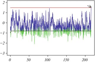
Figure 1 shows two simulated sample paths for the free process Y (t) (green) and for the restricted process X(t) (blue), both obtained via an appropriate algorithm based on the simulation of the Brownian motion in the presence of a constant reflecting boundary and on suitable spatio-temporal transformations (the details of the algorithm are object of our paper in preparation). The arrow in Fig. 1 indicates the instant of the first passage time. The firing pdf g _X[S(t), t | y, τ] is solution of the nonsingular Volterra integral equation (see, [4])