Produces Well Behaved Oscillations and Synchrony

where V is the membrane potential, with V_r and V_t being the resting and threshold values respectively. C is the capacitance of the cell membrane. τ is the membrane time constant such that τ = RC with R being the resistance. I represents a depolarizing input current to the neuron.

2.2 Izhikevich Neurons

The Izhikevich (IZ) neuron model [5] is a two variable system that can model both Type I and Type II neurons depending upon how it is parameterized. The time evolution of the model is defined as follows:

$\frac{\it dV}{\it dt}=0.04{V}^2+5v+140-U+I$
$\frac{\it dU}{\it dt}=a\left( \it bV-U\right)$

if V > 30, then {V ← c, U ← U + d

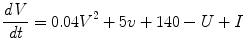
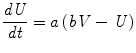
I is the input to the neuron. V and U are the voltage and recovery variable respectively, and a, b, c and d are dimensionless parameters. The chosen parameter values dictate that the Izhikevich neurons used in this paper are Type II neurons with a saddle node bifurcation.

2.3 Hodgkin-Huxley Neurons

The Hodgkin-Huxley (HH) model [6] is a Type II neuron with an Andronov-Hopf bifurcation. Hodgkin and Huxley found three different types of ion current: sodium (Na+), potassium (K+), and a leak current that consists mainly of chloride (Cl-) ions. From their experiments, Hodgkin and Huxley formulated the following equation defining the time evolution of the model:

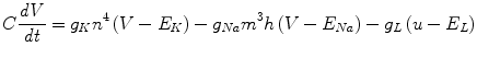
$C\frac{\it dV}{\it dt}={g}_K{n}^4\left(V-{E}_K\right)-{g}_{Na}{m}^3h\left(V-{E}_{Na}\right)-{g}_L\left(u-{E}_L\right)$

C is the capacitance and n, m and h describe the voltage dependence opening and closing dynamics of the ion channels. The standard parameterisation and rate functions for each chemical and channel are used and can be found in Hodgkin and Huxley’s book [6].

2.4 Synaptic Model

A conductance synaptic model is used for experiments using the QIF and IZ models model, whereas the HH model uses synaptic reversal potentials to further scale incoming spikes. The latter model is as follows:

${I}_j(t)={\sum}_i{w}_{ij}{t}_i\left( Rev-{V}_j\right)$

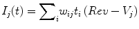where I_j(t) is the input to neuron j at time t, t _i is the spike from neuron i arriving at time t, and w _ij is the weight of the synapse connecting the two neurons. Rev is the reversal potential and V_j is the voltage of the target neuron.

2.5 Spike Timing Dependent Plasticity

The STDP update method used in this paper is an ‘additive nearest neighbour’ scheme. A pre-synaptic spike followed by a post-synaptic spike potentiates the synaptic weight, where as a post-synaptic spike followed by a pre-synaptic spike depresses the weight. The change in weight (Δw) is affected by the exponential of the time difference (Δt) and the learning rate constant (λ):

$\Delta w=\lambda e\frac{-\left|\Delta t\right|}{\tau }$

For potentiation, the learning rate value λ is 0.3, and the window τ is 20 ms. For depression, the learning rate value λ is 0.3105 and the window τ is 10 ms.

2.6 Evolution of Oscillatory Nodes

The neural architecture for generating oscillations used in this paper is pyramidal inter-neuronal gamma (PING).

Whilst the general PING architecture is well understood, the specific details required for both particular oscillatory frequencies and neuron model varies and involves a large space of parameter values within the general PING framework. In order to obtain these values we used a genetic algorithm. In the present work, all neural populations used an excitatory layer of 200 neurons and an inhibitory layer of 50 neurons. The excitatory layer drives the entire network and so is the only one to receive external input. The networks were wired up with connections between excitatory neurons, between inhibitory neurons, from excitatory to inhibitory neurons, and from inhibitory to excitatory neurons.

The parameters that were evolved were the length in milliseconds of the external stimulus presentation, the synaptic weights and delays, as well as the number of synaptic connections between source and target neurons in each pathway. The amount of time trained for was also an evolved parameter for networks that learnt. Two types of PING architecture networks were investigated. The first learnt a stimulus and then after learning would only oscillate to the learnt stimulus. The second did not use learning and so would oscillate to any input stimuli.

2.7 Synchronisation Metric

We only calculated synchrony amongst the excitatory neuron layers. The spikes of each neuron in each excitatory layer were binned over time, and then a Gaussian smoothing filter was passed over the binned data to produce a continuous time varying signal. Following this, we performed a Hilbert transform on the mean-centred filtered signal in order to identify its phase. The synchrony at time t was then calculated as follows:

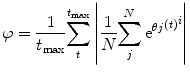$\varphi =\frac{1}{t_{\max }}{\displaystyle \sum_t^{t_{\max }}\left|\frac{1}{N}{\displaystyle \sum_j^N{\mathrm{e}}^{\theta }{{{}^j}^{(t)}}^i}\right|}$

where θ _j(t) is the phase at time t of oscillatory population j. i is the square root of −1. N is the number of oscillators, and t _maxis the length of time of the simulation.

3 Results

3.1 Neuron Model and the Learning of Oscillation

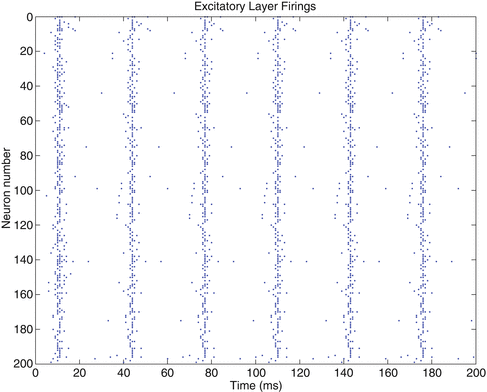
Our first investigation explored how the neuron model affects the ability of a cluster of neurons to learn to oscillate. In order to explore this we evolved neural learning PING oscillators to oscillate at 30 Hz for QIF, IZ and HH neuron models. Figure 1 shows a raster plot of the firings of the excitatory layer from the evolved QIF solution when it has been presented with a learnt stimulus after training. In accord with the finding of Hosaka et al. [2], the network fires regularly at the stimulus presentation, and has narrow and pronounced periodic bands. These thin bands appear approximately every 33 ms giving the 30 Hz oscillation desired.