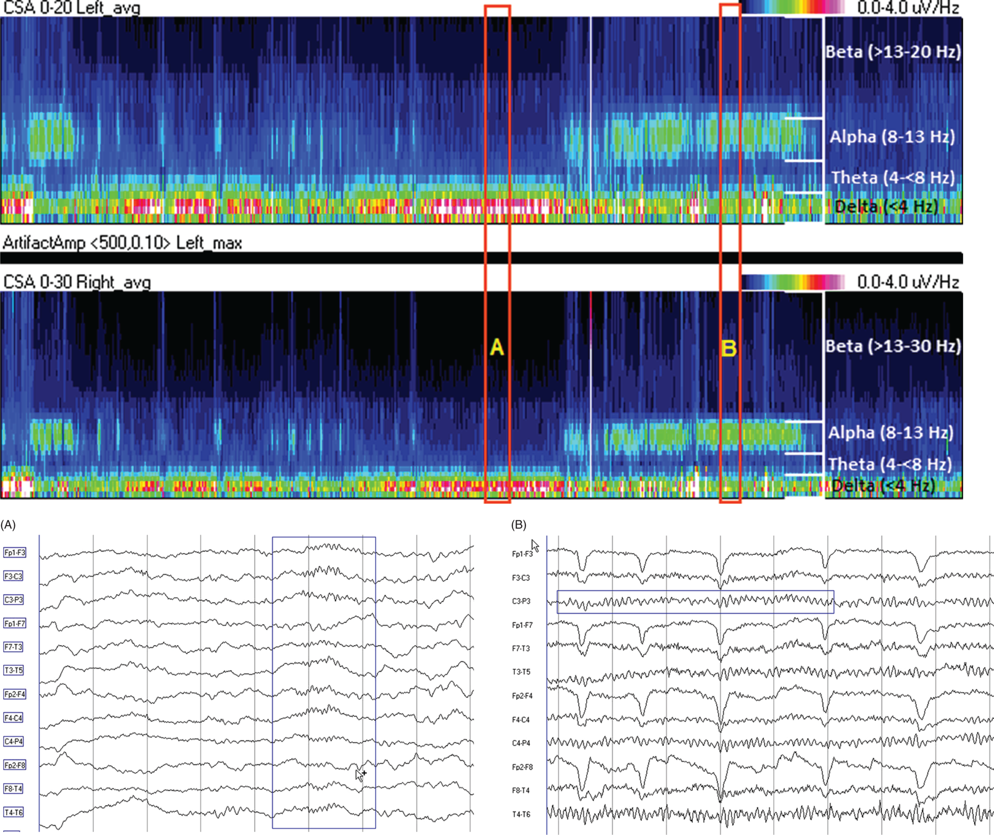
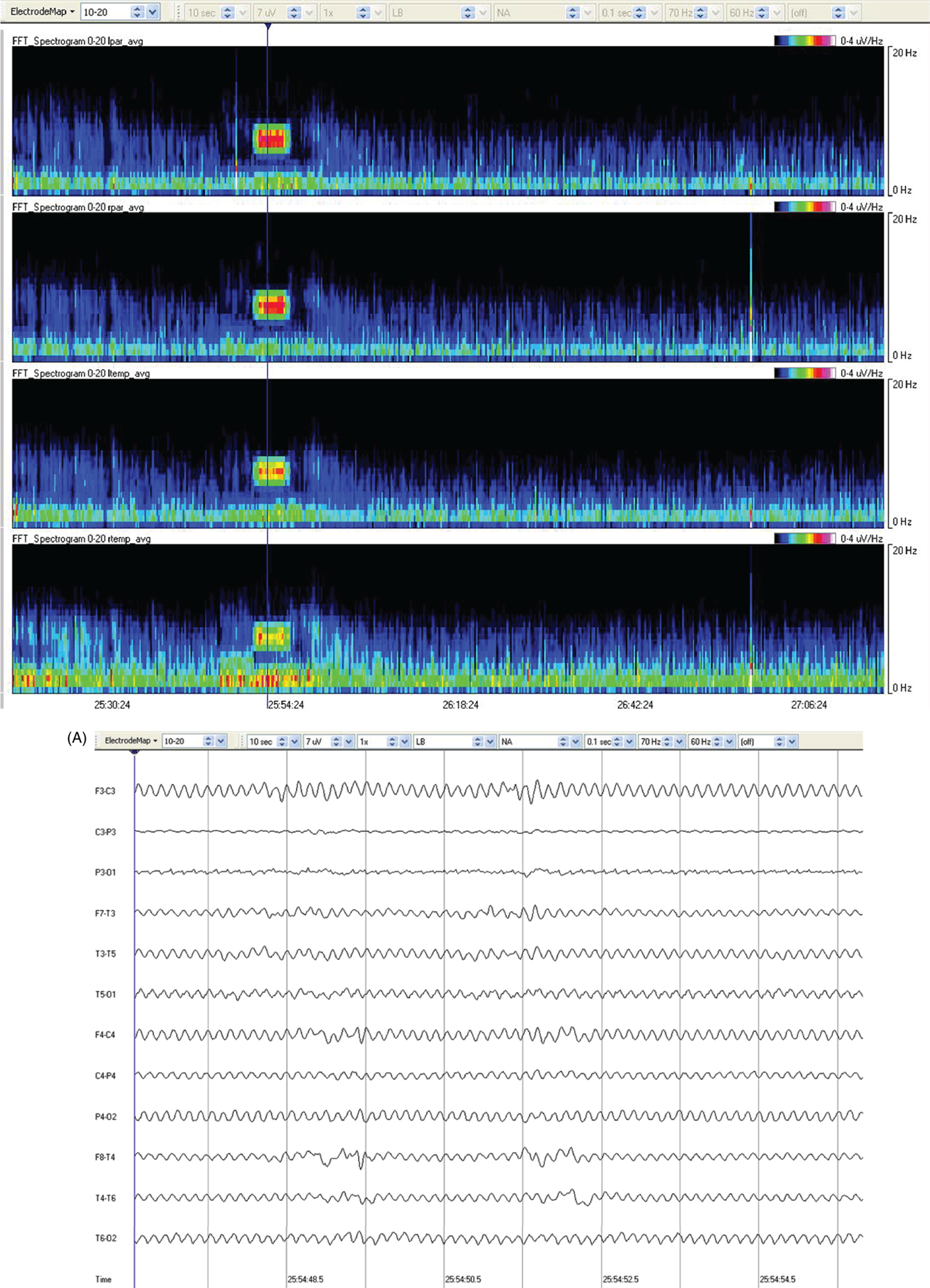
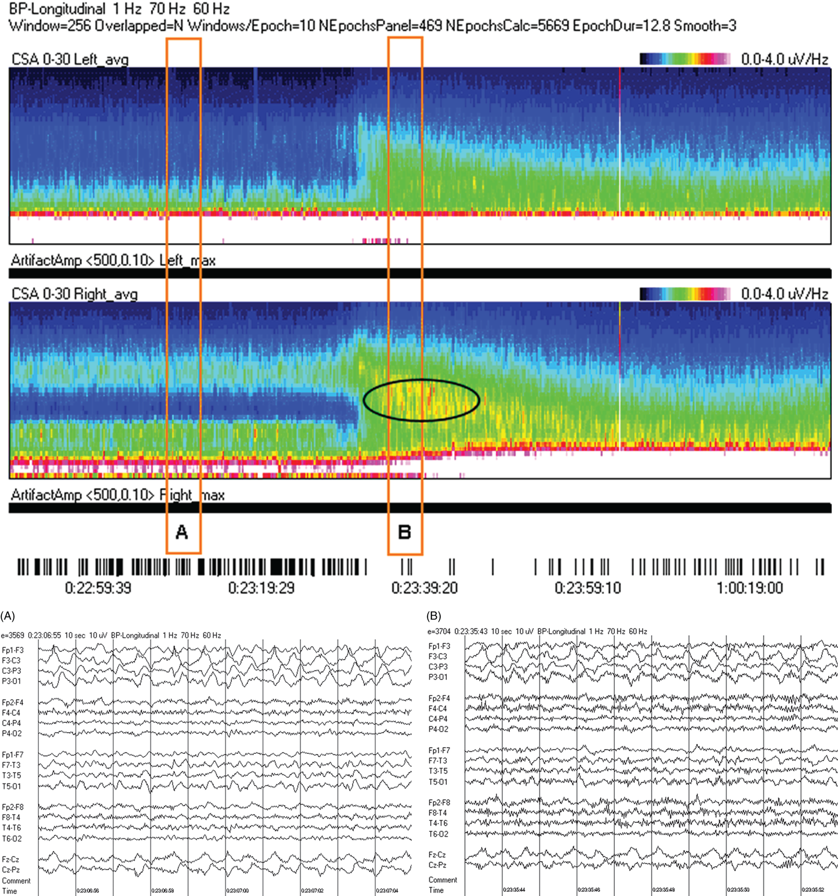
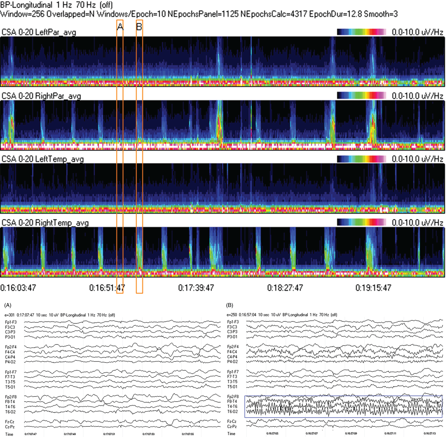
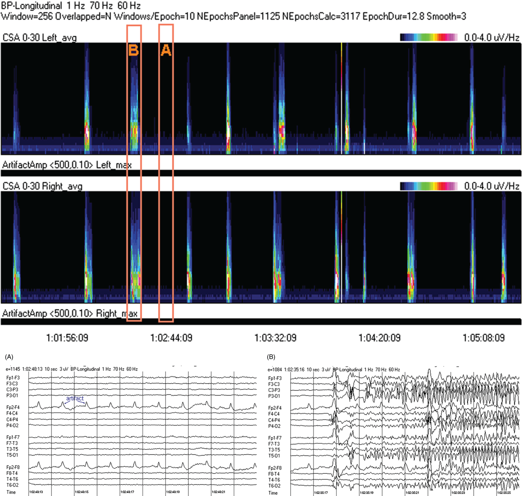
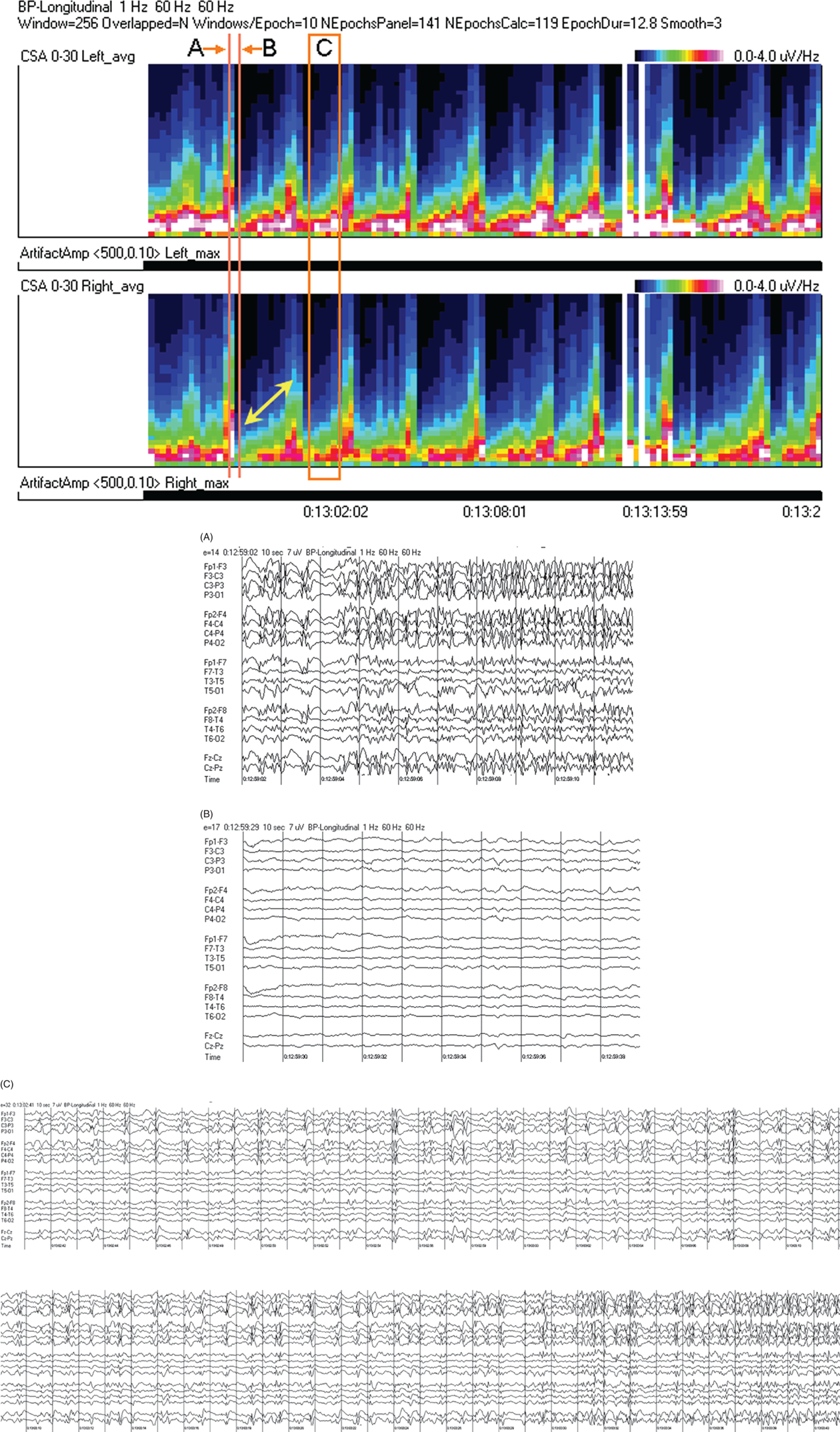
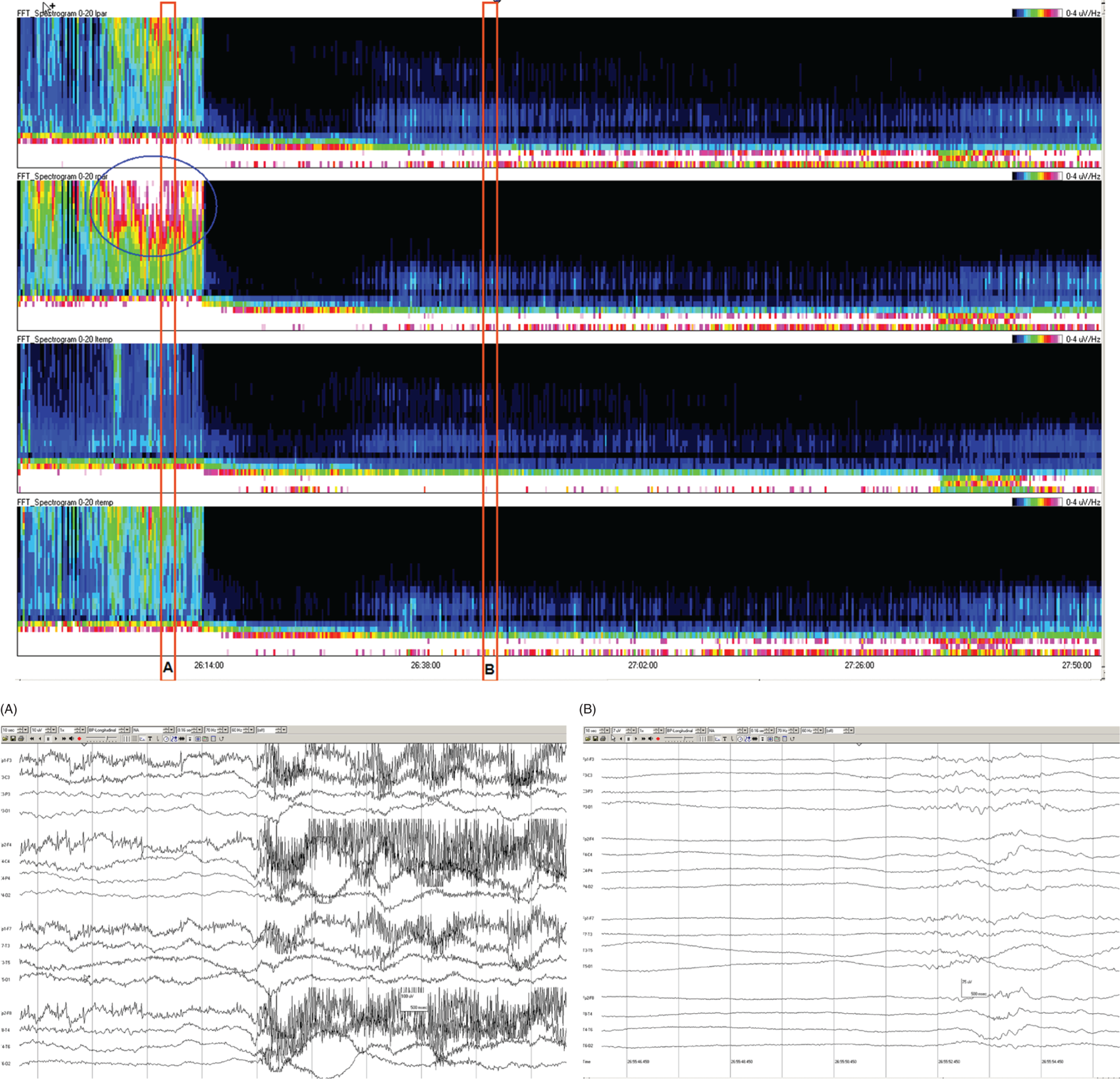
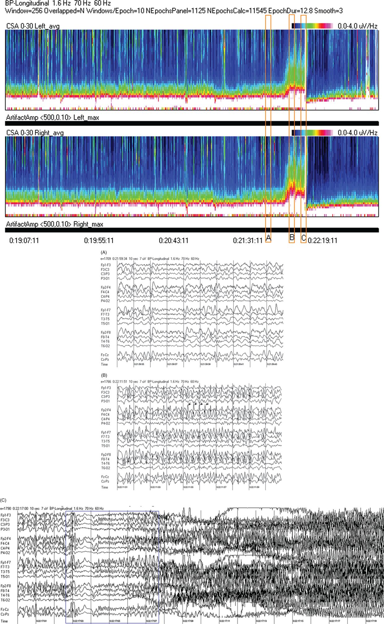
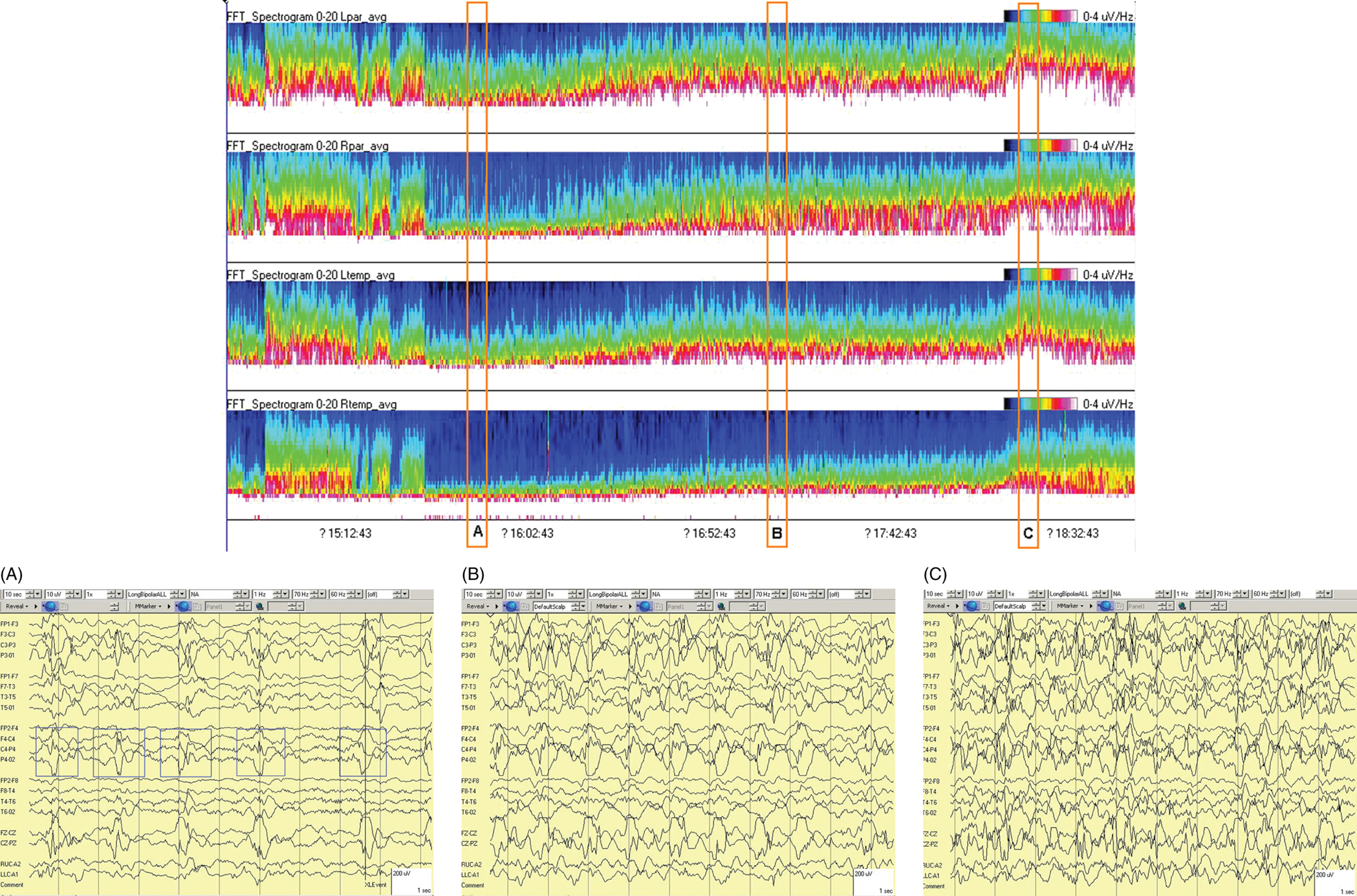
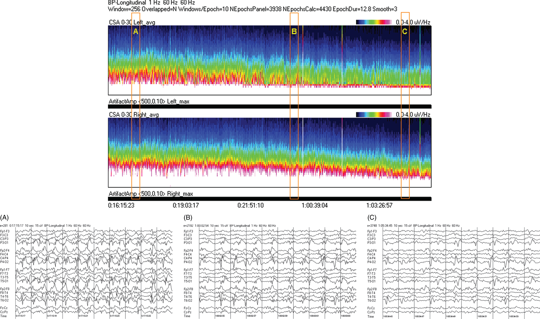
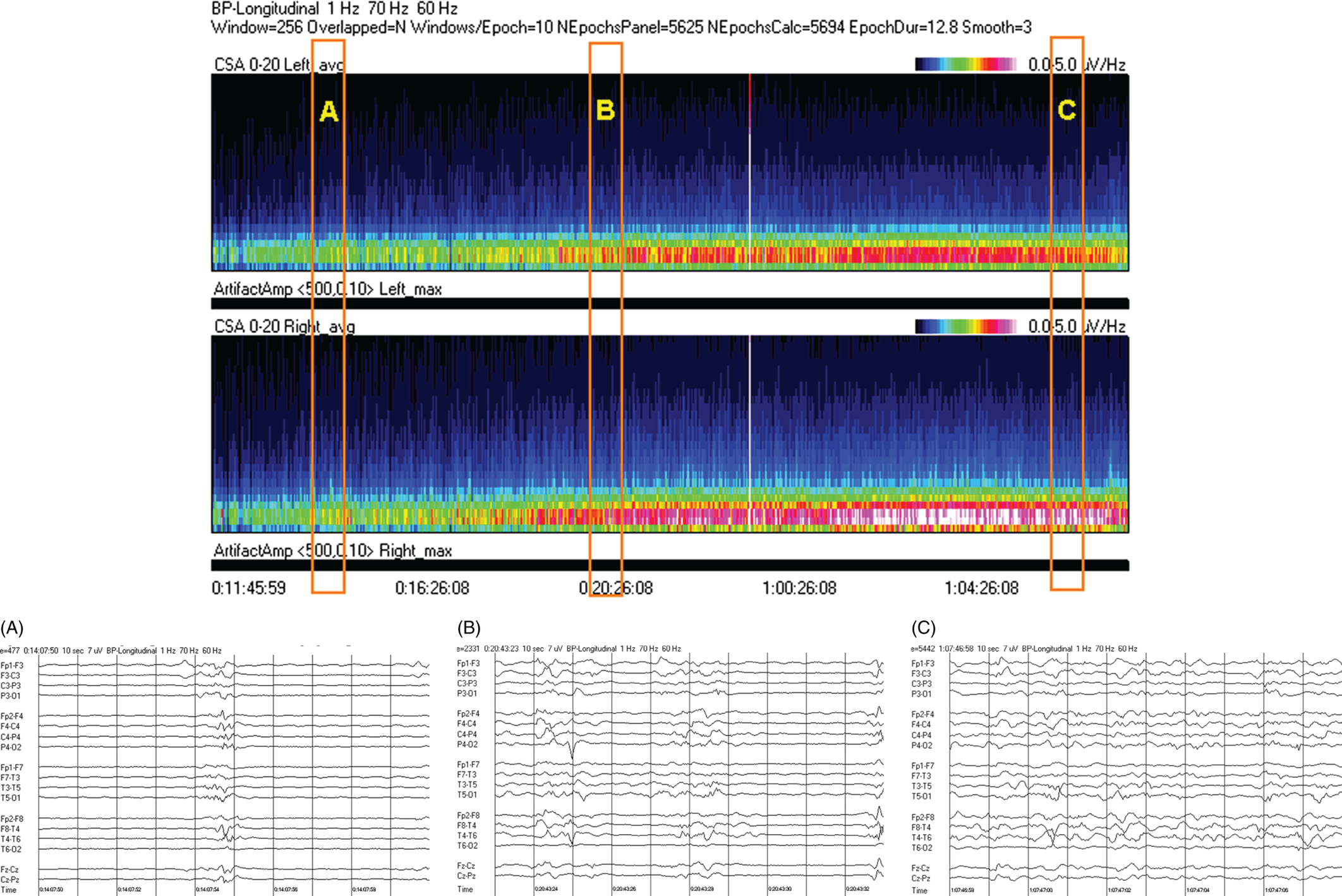
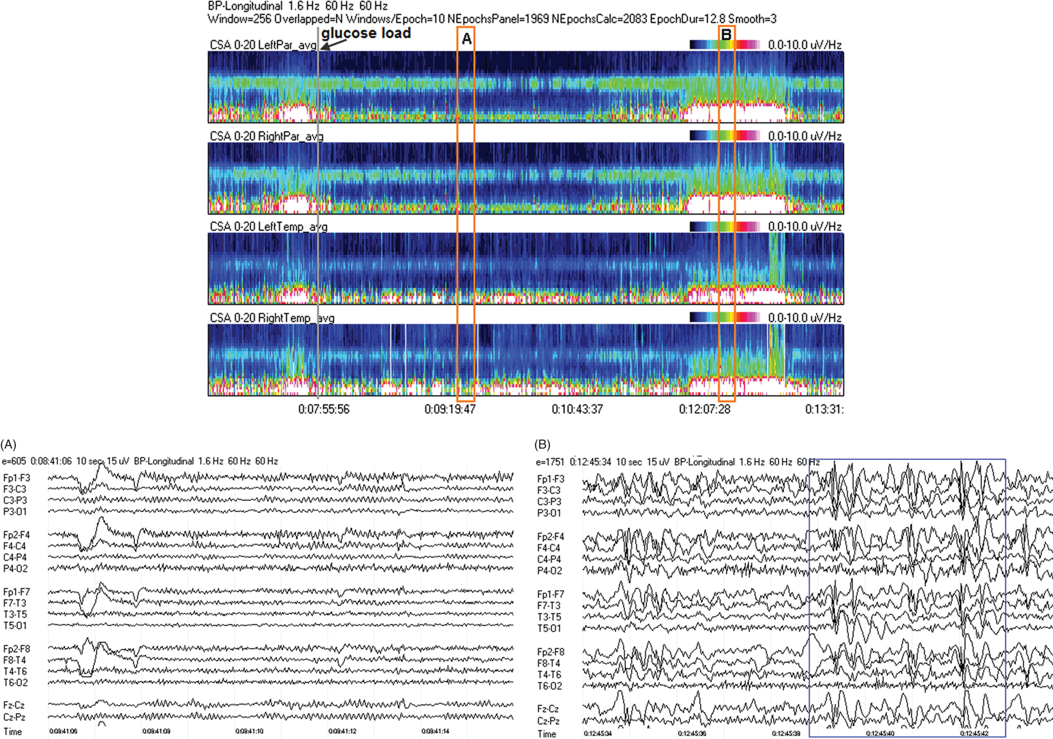
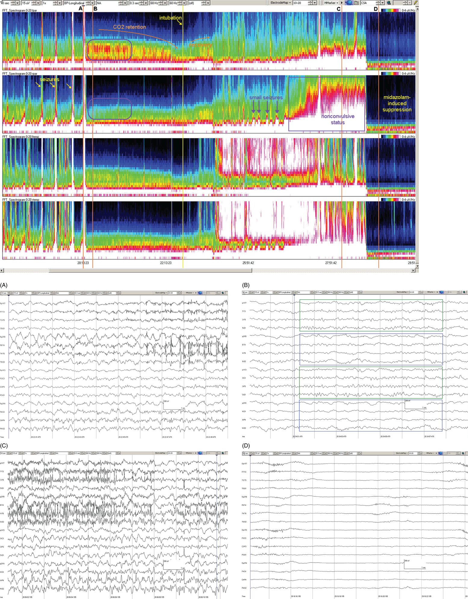
Due to technical advances and increased awareness of the high prevalence of nonconvulsive seizures, prolonged EEG recording in the critically ill is standard of care in many centers. It is clear that the majority of seizures in the intensive care unit are nonconvulsive and can only be recognized with EEG. It is also clear that it is labor-intensive to review these studies. Quantitative EEG techniques have helped immensely in speeding this up. Although many are intimidated by these techniques, they are actually quite simple in principle and easy to learn. As software programs have improved, QEEG has become more and more useful. Not only can seizures be detected, but other acute brain events as well, such as ischemia, hydrocephalus, hemorrhage and so on. Several existing software programs will enable one to set alarms and, theoretically, to do true real-time monitoring once the infrastructure has been put in place and someone is available to respond to the alarms and interpret the study (currently only possible in a small percent of institutions). In the not-too-distant future, this type of real-time monitoring, or ‘neurotelemetry’, will be available in many centers, akin to cardiac telemetry today. This chapter covers the initial basics of quantitative EEG with some of the special indications and uses outlined in a subsequent chapter. Perhaps the simplest way to consider QEEG is to think of it as an additional montage. As introduced in the very first chapter of this book, selecting a different montage does not change the content of the EEG, but rather how this content is displayed. QEEG merely has the advantage of being able to display hours and even days of EEG on a single page. As previously introduced, different montages (or ‘trends’, the term commonly used with QEEG) have strengths and weaknesses, and this concept also applies to the use of QEEG. The QEEG can be thought of as a Swiss army knife. As a whole it is immensely versatile. However, the ability to apply it to every situation depends on the understanding of the range of unique tools that it contains. This chapter aims to introduce the abilities of QEEG, demonstrate certain limitations, and most importantly demonstrate how these limitations can often be overcome by knowledge-based selection of a trend best suited to the task. Quantitative EEG is excellent for detecting seizures, rhythmic and periodic patterns, asymmetries, and for following long-term trends, as discussed in this chapter. The use of QEEG can reduce review times by up to 80% compared to manual screening of the raw EEG, while maintaining good (but not perfect) sensitivity. This can be achieved with appropriate training at a resident level and is easy to incorporate into regular EEG review. Automated seizure detection algorithms have also improved over time and are now at the stage of demonstrating non-inferiority compared to expert review in some studies. The gold standard remains review of the raw EEG; however, QEEG can drastically reduce the time this takes, can highlight subtle features such as asymmetries that can be hard to appreciate, and can easily demonstrate long-term trends, which are often hard to register if looking at the EEG page by page. In addition, it allows detailed, focused review of times of interest (especially times of changing EEG patterns or automated detections) rather than superficial review of all times (as occurs with rapid review of the entire raw EEG). QEEG is particularly useful in monitoring for ischemia; such special applications will be covered in Chapter 10. EEGs throughout this atlas have been shown with the following standard recording filters unless otherwise specified: LFF 1 Hz, HFF 70 Hz, notch filter off. Figure 9.1. Spectrogram basics: state changes and alpha rhythm Figure 9.1main Four hours of normal EEG. A basic and very useful quantitative EEG (QEEG) trend is the Compressed Spectral Array (CSA), which is also referred to as the Fast Fourier transform (FFT), density spectral array (or even compressed density spectral array), or power spectrogram (‘spectrogram’ for short). The premise of the CSA or FFT is that the raw EEG is made up of a series of superimposed rhythms of varying frequencies (delta, theta, alpha, beta, etc.). A Fourier transform can assist with breaking down that EEG into its products. It does this by matching how much of a specific frequency is present at any given time and represents this absolute amount on a color scale. The color scale can be seen at the top right of each row. On the left of the scale, black represents no activity, green the middle and red a high amount of activity. This ‘amount of activity’ is termed ‘power’, and it is akin to area under the curve for activity in that frequency (a combination of amplitude and duration). Within each row, frequency is mapped on the y axis, and time on the x axis. The bottom of the y axis is zero or 1 Hz, and the top of the y axis is typically set between 20–30 Hz (i.e., beta range activity). The scale for the y axis has been superimposed to the right of both rows. The top panel on this page is the CSA for the left hemisphere and the bottom panel the CSA for the right hemisphere. While the patient is asleep (A), most power is in the delta frequency (near the bottom). While awake (B), there is less delta (the white and red are no longer seen at the bottom of the tracings, and there is a prominent horizontal green band at ∼10 Hz. The 10 Hz activity is due to the alpha rhythm (see raw EEG). Note, to demonstrate the effect of altering the scale of the y axis, the top row [left hemisphere] is displaying 0–20 Hz and the bottom row [right hemisphere] is displaying 0–30 Hz (therefore there is more black at the top of the lower row because there is little activity in the 20–30 Hz range that has been omitted from the top row). In practice the y scales of the left and right hemisphere should be equal so a comparison can be easily made between hemispheres. (A) EEG at A: normal stage N2 sleep with a sleep spindle shown in the box. (B) EEG at B: normal awake EEG with a 9.5–10 Hz posterior dominant (alpha) rhythm (box). Figure 9.2. Spectrogram basics: mechanical artifact – bed oscillator Figure 9.2main Spectrogram showing 3 hours of QEEG. The concept of the CSA is highlighted by this example. A pair of CSA rows usually comprises of homologous brain regions (in order to make direct comparison). In Figure 9.1, the left and right hemispheres were being compared. In this example, the top two rows are the left and right parasagittal regions (labels in the top left of each row) and the bottom pair of rows are the left and right temporal regions. Throughout this 3-hour period, the EEG demonstrates diffuse slow activity (with mostly delta, especially <2 Hz, and some theta range power) with no faster frequencies (no power above 10 Hz here, and little above 5–6 Hz). There is then a period lasting several minutes with sudden appearance of activity between 5 and 10 Hz, remaining constant, then stopping suddenly (cursor line is during this activity). This causes a square shape on the spectrogram. Raw EEG at that time shows widespread 7 Hz activity. This was caused by the bed vibrating at 7 Hz due to a mechanical oscillator. Sharp edges on a spectrogram (sudden on, sudden off) and a constant frequency activity (perfectly flat tops and bottoms) with little change should raise suspicion of mechanical artifact. The example highlights the concept of the CSA: when a 7 Hz activity is suddenly introduced into the EEG, there is a high amount of power seen at this specific frequency. The activity is unchanging, and therefore the red band remains as long as the artifact is present. As soon as it is turned off, there is very little power in this frequency, and therefore the band instantly disappears. (A) EEG at line showing a monomorphic sinusoidal 7-Hz activity from a bed oscillator. Figure 9.3. Spectrogram basics: drug-induced beta and asymmetry Figure 9.3main Two hours of QEEG demonstrating the spectrogram between 1–30 Hz in a 4-year-old with status epilepticus (with right body twitching at times), treated with midazolam infusion. The case demonstrates the benefit of viewing homologous brain regions. At the beginning of the record there is a clear asymmetry with slowing (more delta power) and attenuation (less power in alpha/beta ranges) on the left (A). A benzodiazepine bolus (midazolam) is then administered, and a marked increase in fast activity can be seen (B), still somewhat greater on the right (where the power in the alpha band reaches yellow and even red at times; ellipse) (the healthier side). There is also an increase in the delta power on the right side, matching the left (white band at the bottom) as the patient becomes sedated. (A) EEG at A: marked left-sided slowing, maximal parasagittally, consisting of high amplitude, continuous 1–2 Hz delta (this explains the very high delta power at the beginning of the record: continuous and high amplitude = very high power). There is attenuation of normal faster activity on the left as well, but faster frequencies are fairly prominent on the healthier right side. (B) EEG at B: much more fast activity (enhanced beta), a common effect of benzodiazepines and barbiturates; this is increased on both sides, but still asymmetric (more on the right). Note the left hemisphere is very slow (high delta power); because of this it is difficult to appreciate an increase/change in the delta power in that hemisphere following benzodiazepine. What is appreciated is that the right hemisphere has become proportionately much slower when compared to before benzodiazepine. This difference can be easily appreciated on the spectrogram, and the delta power at the end of the epoch looks fairly similar to that in the left. Figure 9.4. Spectrogram basics: multiple seizures. Figure 9.4main Four hours of EEG in a young woman with an unusual leukodystrophy (ovarioleukodystrophy) and intractable nonconvulsive seizures. This quantitative EEG (QEEG) sample shows time along the x axis (4 hours shown), frequency on the y axis (0–20 Hz, which can be found in the top left of each row), and power in the z axis, with power shown on a color scale where the highest power is white, followed by pink and red (see color scales in the upper right of each panel). There are four rows shown in this QEEG panel, representing different electrode chains (left parasagittal, right parasagittal, left temporal, right temporal). Most power is near the bottom in the delta range for most of the tracing. There are intermittent bursts of power in higher frequencies on the right, usually maximal in the temporal region; one example is shown in B. These represent seizures, although review of the raw EEG at that point is necessary to confirm this. QEEG should never be interpreted without reviewing portions of the original waveforms as well. Ictal patterns have this characteristic shape on a spectrogram with the sudden increase of power through higher frequencies and then sudden decline to baseline; this appearance is sometimes called ‘flames’. Additional examples of flames with a full QEEG panel can be found in figures 9.21 and 9.22. (A) EEG at A: baseline, showing diffuse delta activity. (B) EEG at B: right temporal seizure (box). Figure 9.5. Spectrogram basics: multiple seizures arising from complete suppression Figure 9.5main Six hours of QEEG in a 12-year-old boy with refractory status epilepticus being treated with pentobarbital coma. The background was completely suppressed (A) with no bursts, yet well-developed seizures still occurred about twice per hour (B). Note, at point A the spectrogram is mostly black apart from a very faint signal in the low delta band. This is typical of complete suppression, i.e., there is no power in any frequency, with some delta power being registered due to artifact. This example demonstrates the limitations of intermittent short EEGs for monitoring barbiturate-induced coma, which would miss seizures if a short EEG was done at the time of suppression. (A) EEG at A: interictal, showing complete suppression and Fp2 artifact. Sensitivity 3 uV/mm (high gain). (B) EEG at B: start of a seizure, beginning maximally on the left, but rapidly becoming bilateral. Figure 9.6. Spectrogram basics: cyclic nonconvulsive seizures. Figure 9.6main ∼30 minutes of QEEG in a middle-aged woman with encephalitis, seizures and brief cardiac arrest. Brief nonconvulsive seizures were occurring every ∼3 minutes in a very stable pattern of seizure (A), postictal attenuation (B), then gradual buildup of epileptiform activity (yellow arrow and C) until another seizure occurs. (A) EEG at A: definite electrographic seizure, maximal in bilateral parasagittal chains. (B) EEG at B: postictal, with marked diffuse attenuation. (C) One minute of raw EEG at C: gradual buildup of epileptiform activity between seizures. Figure 9.7. Spectrogram basics: muscle artifact Figure 9.7main Two hours of EEG showing an initial period with prominent muscle artifact, maximal in the right parasagittal region (blue ellipse). Muscle artifact on a spectrogram tends to appear as if it is coming down from the top (stalactites) of the tracing (as in this example). This is because EMG artifact is usually composed primarily of frequencies greater than those being displayed (>20 Hz in this example). A sample of EEG during this time period is shown at point A. There is then a period with no muscle artifact and with most power in the lower frequencies, corresponding to sleep (point B). (A) EEG at A: awake recording with prominent muscle artifact, maximal in the right parasagittal region as seen on the spectrogram. (B) EEG at B: sleep recording with no muscle artifact. Figure 9.8. Spectrogram basics, long-term trends: NCSE culminating with convulsion Figure 9.8main Four hours of QEEG power spectrograms (CSA) from a middle-aged man with genetic generalized epilepsy and seizures since age 9, now admitted with intermittent confusion. Baseline EEG (point A) shows diffuse slowing. He then develops nonconvulsive status epilepticus for 15–20 minutes (point B), which continues until he develops a generalized tonic-clonic seizure (point C). There is brief post ictal attenuation after this point. (A) EEG at A: diffuse slowing with no definite ictal activity. (B) EEG at B: nonconvulsive status epilepticus (NCSE), with irregular, ∼3 Hz generalized spike-wave. Arrows highlight a few of the spikes. (C) EEG at C: transition from NCSE (first few seconds) into a typical generalized tonic-clonic seizure. Figure 9.9. Spectrogram basics, long-term trends: slow worsening ictal-interictal continuum (IIC) progressing to electrographic status epilepticus (ESE). Figure 9.9main Power spectrogram showing 4 hours of EEG in a 4-month-old boy with refractory nonconvulsive seizures. Although treatment had stopped NCSE just prior to point A, the ictal pattern gradually resumed and worsened over the next several hours. This is a good example of the IIC. There is no clear demarcation and no clear and abrupt transition from interictal to ictal states. Instead (as is often the case in critically ill patients) there is a gradual, smooth transition from one to the other. (A) EEG at A: periodic complexes every 1.5–2 seconds (boxes), bisynchronous and maximal in the parietal regions (LPDs, bilateral asymmetric). This is most likely not an ictal pattern. (B) EEG at B: higher amplitude complexes (sensitivity is at 10 uV/mm), more epileptiform and faster, now at 1 Hz and with more superimposed fast frequencies (LPDs+F, high amplitude). This is not definite electrographic seizure activity (but on the ictal end of the ictal-interictal continuum), but we would consider this to be probably ictal at this point, though the exact point that interictal became ictal is not well defined. (C) EEG at C: even higher amplitude and continuous epileptiform activity including fast frequencies, which is unequivocally an ictal EEG pattern at this point. There was no clear clinical correlate (electrographic status epilepticus [ESE]). Figure 9.10. Spectrogram basics, long-term trends: gradual resolution of ESE, IIC and BIPDs Figure 9.10main Twelve-hour spectrogram in a 3-year-old s/p cardiac surgery showing gradual resolution of NCSE/ESE. This example also supports the concept of an ictal-interictal continuum as this patient has smooth, gradual transition from probably ictal to interictal, with no clear cutoff point. (A) EEG at A: posterior-predominant, ∼1.5 Hz high amplitude (note sensitivity is at 15 μV/mm) periodic discharges, mostly but not always bisynchronous, often polyspike-and-wave morphology. This pattern is on the ictal-interictal continuum, arguably ictal at this point. (B) EEG at B: similar pattern, but a bit slower, with brief breaks in the rhythmicity for half a second or so, and with more restricted field and more evidence of a bilateral independent pattern. These are BIPDs+F and still on the ictal-interictal continuum, although clearly improved (much less likely to be ictal) compared to earlier in the record. (C) EEG at C: BIPDs with both populations now at < 1 Hz and with resolution of the plus F. Now clearly not ictal at this point. Figure 9.11. Spectrogram basics, long-term trends: wearing off of pentobarbital Figure 9.11main Spectrogram showing about 20 hours of EEG during pentobarbital-induced coma in a 6-month-old boy with a left frontal hemorrhagic infarct and refractory status epilepticus. By showing this many hours of EEG at once, it is easy to appreciate the long gradual wearing off of the pentobarbital effect. The suppression percent or amplitude-integrated EEG would be additional good QEEG methods for following this (see Figures 9.14 and 9.15). (A) EEG at A: suppression-burst, with just one short burst on this 10 second page. (B) EEG at B: suppression-burst, with more frequent bursts. (C) EEG at C: emergence out of suppression-burst. Figure 9.12. Spectrogram basics, long-term trends: glucose load effect in glucose transporter deficiency. Figure 9.12main Nine hours of QEEG power spectrograms (CSA) in a child with glut-1 deficiency syndrome, a condition with low CSF glucose due to a defect in the glucose transporter glut-1, which transports glucose into the central nervous system across the blood-brain barrier. Many patients with this syndrome have seizures and generalized epileptiform discharges. This example shows periods of high delta power due to frequent generalized spike-wave discharges (before the glucose load, and much later in the record at point B). These resolve with a glucose load (labeled line) and the EEG normalizes (point A). After fasting for 5–6 hours, the generalized epileptiform discharges gradually return (point B). (A) EEG at A: no epileptiform discharges. (B) EEG at B: frequent irregular generalized spike-wave discharges (box), resulting in marked increase in delta power (due to the high voltage delta waves associated with the spikes). Figure 9.13. Spectrogram basics, long-term trends: CO2 retention, acidosis and resolution of nonconvulsive seizures
9
Quantitative EEG: basics, seizure detection and avoiding pitfalls
Figure list
9.1 Spectrogram basics
9.2 Quantitative EEG: basics
9.3 Quantitative EEG: detection of seizures and rhythmic and periodic patterns
9.4 Quantitative EEG: pitfalls and solutions
Suggested reading
Stay updated, free articles. Join our Telegram channel

Full access? Get Clinical Tree


