. In neural systems, these parameters usually correspond to time constants or synaptic strengths of the connections between the system elements. The mathematical form of the dependencies  and the pattern of absent and present connections represent the structure of the system. Each element of the system or region is then driven by some endogenous or subcortical input u. We can therefore write down a general state equation for non-autonomous deterministic systems in the following manner,

(1)
A model whose form follows this general state equation provides a causal description of how system dynamics result from system structure, because it describes (i) when and where external inputs enter the system; and (ii) how the state changes induced by these inputs evolve in time—depending on the system’s structure. Given a particular temporal sequence of inputs u(t) and an initial state x(0), one obtains a complete description of how the dynamics of the system (i.e. the trajectory of its state vector in time) results from its structure by integration of the general state equation. It provides in this way, a general form for models of effective connectivity in neural systems.
In the DCMs considered in this chapter, we assume that all processes in the system are deterministic and occur instantaneously. Whether or not this assumption is valid depends on the particular system of interest. If necessary, random components (noise) and delays can be accounted for by using stochastic differential equations and delay differential equations, respectively. We also assume that we know the inputs that enter the system. This is a tenable assumption in neuroimaging because the inputs are experimentally controlled variables, e.g. changes in stimuli or instructions. It may also be helpful to point out that using time-invariant dependencies F and parameters θ does not exclude modelling time-dependent changes of the network behaviour. Although the mathematical form of F per se is static, the use of time-varying inputs u allows for dynamic changes in what components of F are ‘activated’. Also, there is no principled distinction between states and time-invariant parameters. Therefore, estimating time-varying parameters can be treated as a state estimation problem.
This approach regards an experiment as a designed perturbation of neuronal dynamics that are promulgated and distributed throughout a system of coupled anatomical nodes to change region-specific neuronal activity. These changes engender, through a measurement-specific forward model, responses that are used to identify the architecture and time constants of the system at a neuronal level. An important conceptual aspect of dynamic causal models pertains to how the experimental inputs enter the model and cause neuronal responses.
DCM using Convolution Based Models
In this section, we provide a brief review of DCM with convolution based models. For more details about convolution-based models we refer the reader to [3, 12, 29–32]. In general, the aim of DCM is to estimate, and make inferences about (i) the coupling among brain areas, (ii) how that coupling is influenced by experimental changes (e.g. time or cognitive set) and (iii) what are the underlying neurobiological determinants that can account for the variability of observed activity. Crucially, one constructs a reasonably realistic neuronal model of interacting cortical regions or nodes and supplements this with a forward model of how neuronal or synaptic activity translates into a measured response. This enables the parameters of the neuronal model (e.g., effective connectivity) to be estimated from observed data. This process is the same for both the convolution models discussed in this section and the conductance based models discussed in later sections. Electrophysiology has been used for decades as a measure of perceptual, cognitive operations, etc [36, 37]. However, much remains to be established about the exact neurobiological mechanisms underlying their generation [38–40]. DCM for ERPs was developed as a biologically plausible model to understand how event-related responses result from the dynamics in coupled neural ensembles. It rests on a neural mass model which uses established connectivity rules in hierarchical sensory systems to assemble a network of coupled cortical sources. This kind of neural-mass model has been widely used to model electrophysiological recordings (e.g., [41–47] and has also been used as the basis of a generative model for event-related potentials and induced or steady-state responses that can be inverted using real data [3, 4, 23, 48–50].
The DCM developed in [3], uses the connectivity rules described in [51] to model a network of coupled sources. These rules are based on a partitioning of the cortical sheet into supra-, infra-granular layers and granular layer (layer IV). Generally speaking, bottom-up or forward connections originate in agranular layers and terminate in layer IV. Top-down or backward connections target agranular layers. Lateral connections originate in agranular layers and target all layers. These long-range or extrinsic cortico-cortical connections are excitatory and arise from pyramidal cells.
Each region or source is modelled using a neural mass model described in [32], based on the model of [44]. This model emulates the activity of a cortical area using three neuronal subpopulations, assigned to granular and agranular layers. A population of excitatory pyramidal (output) cells receives inputs from inhibitory and excitatory populations of interneurons, via intrinsic connections (intrinsic connections are confined to the cortical sheet). Within this model, excitatory interneurons can be regarded as spiny stellate cells found predominantly in layer IV and in receipt of forward connections. Excitatory pyramidal cells and inhibitory interneurons are considered to occupy agranular layers and receive backward and lateral inputs (see Fig. 3.1).
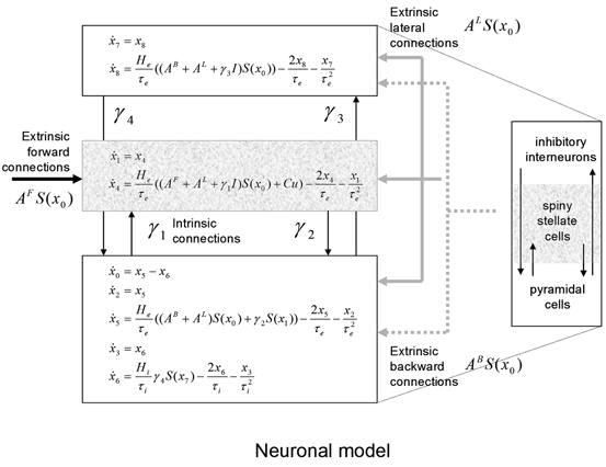

Fig. 3.1
Convolution-based neural mass model. Schematic of the DCM used to model electrophysiological responses. This schematic shows the state equations describing the dynamics of sources or regions. Each source is modelled with three subpopulations (pyramidal, spiny stellate and inhibitory interneurons) as described in [32, 44]. These have been assigned to granular and agranular cortical layers which receive forward and backward connections respectively [3]
To model event-related responses, the network receives inputs via input connections. These connections are exactly the same as forward connections and deliver inputs to the spiny stellate cells in layer IV. The vector C controls the influence of the input on each source. The lower, upper and leading diagonal matrices  encode forward, backward and lateral connections respectively. The DCM here is specified in terms of the state equations shown in Fig. 3.1 and a linear output equation
 encode forward, backward and lateral connections respectively. The DCM here is specified in terms of the state equations shown in Fig. 3.1 and a linear output equation
(2)
where  represents the trans-membrane potential of pyramidal cells and L is a lead field matrix coupling electrical sources to the EEG channels [52].
 represents the trans-membrane potential of pyramidal cells and L is a lead field matrix coupling electrical sources to the EEG channels [52].
Within each subpopulation, the evolution of neuronal states rests on two operators. The first transforms the average density of pre-synaptic inputs into the average postsynaptic membrane potential. This is modelled by a linear transformation with excitatory and inhibitory kernels parameterised by  and
and  .
.  control the maximum post-synaptic potential and
  represent a lumped rate-constant. The second operator S transforms the average potential of each subpopulation into an average firing rate. This is assumed to be instantaneous and is a sigmoid function. Interactions, among the subpopulations, depend on constants
  , which control the strength of intrinsic connections and reflect the total number of synapses expressed by each subpopulation. Having specified the DCM in terms of these equations one can estimate the coupling parameters from empirical data using a standard variational Bayesian scheme, under a Laplace approximation to the true posterior [53]. This is known as Variational Laplace.
 and
and  .
.  control the maximum post-synaptic potential and
  represent a lumped rate-constant. The second operator S transforms the average potential of each subpopulation into an average firing rate. This is assumed to be instantaneous and is a sigmoid function. Interactions, among the subpopulations, depend on constants
  , which control the strength of intrinsic connections and reflect the total number of synapses expressed by each subpopulation. Having specified the DCM in terms of these equations one can estimate the coupling parameters from empirical data using a standard variational Bayesian scheme, under a Laplace approximation to the true posterior [53]. This is known as Variational Laplace.
DCM Using Neural Mass and Mean Field Models of Ensemble Activity
The use of neuronal models to simulate large networks of neurons has enjoyed recent developments, involving both direct simulations of large numbers of neurons (which can be computationally expensive); e.g., [54] and probabilistic approaches; e.g. [55, 56]. Probabilistic approaches model the population density directly and bypass direct simulations of individual neurons. This (mean field) treatment of neuronal models exploits a probability mass approximation. This effectively replaces coupled Fokker-Planck equations describing population density dynamics, with equations of motion for expected neuronal states and their dispersion; that is, their first and second moments. These equations are formulated in terms of the mean and covariance of the population density over each neuronal state, as a function of time. In other words, an ensemble density on a high-dimensional phase-space is approximated with a series of low-dimension ensembles that are coupled through mean-field effects. The product of these marginal densities is then used to approximate the full density. Critically, the mean-field coupling induces nonlinear dependencies among the density dynamics of each ensemble. This typically requires a nonlinear Fokker-Planck equation for each ensemble. The Fokker-Planck equation prescribes the evolution of the ensemble dynamics, given any initial conditions and equations of motion that constitute the neuronal model. However, it does not specify how to encode or parameterize the density. There are several approaches to density parameterization [56–61]. These include binning the phase-space and using a discrete approximation to a free-form density. However, this can lead to a vast number of differential equations, especially if there are multiple states for each population. One solution is to reduce the dimension of the phase-space to render the integration of the Fokker-Planck more tracTable (e.g., [62]). Alternatively, one can assume the density has a fixed parametric form and deal only with its sufficient statistics [63–65]. The simplest form is a delta-function or point mass; under this assumption one obtains neural-mass models. In short, we replace the full ensemble density with a mass at a particular point and then summarize the density dynamics by the location of that mass. What we are left with is a set of non-linear differential equations describing the dynamic evolution of this mode. In the full nonlinear Fokker-Planck formulation, different phase-functions or probability density moments could couple to each other; both within and between ensembles. For example, the average depolarisation in one ensemble could be affected by the dispersion or variance of depolarisation in another, see [66]. In neural-mass models, one ignores this potential dependency because only the expectations or first moments are coupled. There are several devices that are used to compensate for this simplification. Perhaps the most ubiquitous is the use of a sigmoid function  relating expected depolarisation to expected firing-rate [67, 68]. This implicitly encodes variability in the post-synaptic depolarisation, relative to the potential at which the neuron would fire. This affords the considerable simplification of the dynamics and allows one to focus on the behaviour of a large number of ensembles, without having to worry about an explosion in the number of dimensions or differential equations one has to integrate. Important generalisations of neural-mass models, which allow for states that are function of position on the cortical sheet, are referred to as neural-field models, as we will see later.
 relating expected depolarisation to expected firing-rate [67, 68]. This implicitly encodes variability in the post-synaptic depolarisation, relative to the potential at which the neuron would fire. This affords the considerable simplification of the dynamics and allows one to focus on the behaviour of a large number of ensembles, without having to worry about an explosion in the number of dimensions or differential equations one has to integrate. Important generalisations of neural-mass models, which allow for states that are function of position on the cortical sheet, are referred to as neural-field models, as we will see later.
Conductance Based Models
The neuronal dynamics here conform to a simplified [69] model, where the states  comprise transmembrane potential and a series of conductances corresponding to different types of ion channel. The dynamics are given by the stochastic differential equations
 comprise transmembrane potential and a series of conductances corresponding to different types of ion channel. The dynamics are given by the stochastic differential equations
(3)
They are effectively the governing equations for a parallel resistance-capacitance circuit; the first says that the rate of change of transmembrane potential (times capacitance,  ) is equal to the sum of all currents across the membrane (plus exogenous current,
  ). These currents are, by Ohm’s law, the product of potential difference between the voltage and reversal potential,
  for each type of conductance. These currents will either hyperpolarise or depolarise the cell, depending on whether they are mediated by inhibitory or excitatory receptors respectively (i.e., whether
  is negative or positive). Conductances change dynamically with a characteristic rate constant
  and can be regarded as the number of open channels. Channels open in proportion to pre-synaptic input
  and close in proportion to the number open.
 ) is equal to the sum of all currents across the membrane (plus exogenous current,
  ). These currents are, by Ohm’s law, the product of potential difference between the voltage and reversal potential,
  for each type of conductance. These currents will either hyperpolarise or depolarise the cell, depending on whether they are mediated by inhibitory or excitatory receptors respectively (i.e., whether
  is negative or positive). Conductances change dynamically with a characteristic rate constant
  and can be regarded as the number of open channels. Channels open in proportion to pre-synaptic input
  and close in proportion to the number open.
Ensemble models of neuronal populations can employ mean-field (MFM) and neural-mass (NMM) approximations. Ensemble models (Eq. 3.3) provide the trajectories of many neurons to form a sample density of population dynamics. The MFM is obtained by a mean-field and a Laplace approximation to these densities. The NMM is a special case of the mean-field model in which we ignore all but the first moment of the density (i.e., the mean or mode). In other words, the NMM discounts dynamics of second-order statistics (i.e., variance) of the neuronal states. The mean-field models allow us to model interactions between the mean of neuronal states (e.g., firing rates) and their dispersion or variance over each neuronal population modelled (c.f., [70]). The key behaviour we are interested in is the coupling between the mean and variance of the ensemble, which is lost in the NMM. The different models and their mathematical representations are summarised in Table 3.1.
Table 3.1
Comparison of ensemble, Mean-Field (MF) and Neural-Mass (NM) models. The evolution of the Ensemble dynamics decomposes into deterministic flow and diffusion. Those reduce to a simpler MFM form under Gaussian (Laplace) assumptions, where first order population dynamics are a function of flow and the curvature of the flow, and the second order statistics are a function of the gradients of flow. Those reduce to a simpler NMM form by fixing its second order statistics (dispersion) to constant values
Model | Description | Equation |
|---|---|---|
Ensemble | Stochastic differential equation that describes how the states evolve as functions of each other and some random fluctuations |  |
MFM | Differential equation that describes how the mean and covariance of a neuronal populations evolve. This rests on mean-field and Laplace approximations of the ensemble dynamics |  |
NMM | Differential equation that describes how the density evolves as a function of the mean. Obtained by fixing the covariance of the MFM |  |
The three populations of Fig. 3.2 below emulate a source and yield predictions for observed electromagnetic responses. Similarly to the network of Fig. 3.1, each source comprises two excitatory populations and an inhibitory population. These are taken to represent input cells (spiny stellate cells in the granular layer of cortex), inhibitory interneurons (allocated somewhat arbitrarily to the superficial layers) and output cells (pyramidal cells in the deep layers). The deployment and intrinsic connections among these populations are shown in Fig. 3.2.
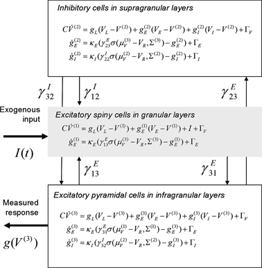

Fig. 3.2
Conductance-based neural mass model. Neuronal state-equations for a source model with a layered architecture comprising three interconnected populations (Spiny-stellate, Interneurons, and Pyramidal cells), each of which has three different states (Voltage, Excitatory and Inhibitory conductances)
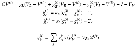
In this model, we use three conductance types: leaky, excitatory and inhibitory conductance. This gives, for each population
(4)
Notice that the leaky conductance does not change, which means the states reduce to  . Furthermore, for simplicity, we have assumed that the rate-constants, like the reversal potentials are the same for each population. The excitatory and inhibitory nature of each population is defined entirely by the specification of the non-zero intrinsic connections
  , see Fig. 3.2.
 . Furthermore, for simplicity, we have assumed that the rate-constants, like the reversal potentials are the same for each population. The excitatory and inhibitory nature of each population is defined entirely by the specification of the non-zero intrinsic connections
  , see Fig. 3.2.
This approach was first applied to FitzHugh-Nagumo (FN) neurons [63, 71] and later to Hodgkin-Huxley (HH) neurons [64, 72]. This approach assumes that the distributions of the variables are approximately Gaussian so that they can be characterized by their first and second order moments; i.e., the means and covariances. In related work, Hasegawa described a dynamical mean-field approximation (DMA) to simulate the activities of a neuronal network. This method allows for qualitative or semi-quantitative inference on the properties of ensembles or clusters of FN and HH neurons; see [65, 73].
Using the three population source from Fig. 3.2 it can be seen that the population responses of the MFM and NMM show clear qualitative differences in dynamic repertoire, with the MFM presenting limit-cycle attractors after bifurcations from a fixed-point [24], which could be useful for modelling nonlinear or quasi-periodic dynamics, like nested oscillations (Fig. 3.3). This produces phase-amplitude coupling, between the inhibitory population and the spiny population that is driven by the low-frequency input. The bursting and associated nested oscillations are caused by nonlinear interactions between voltage and conductance, which are augmented by coupling between their respective means and dispersions.
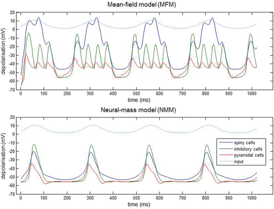

Fig. 3.3
Nested oscillations. Three-population source (Fig. 3.2) driven by slow sinusoidal input for both MFM and NMM. Input is shown in light blue, spiny interneuron depolarization in dark blue, inhibitory interneurons in green and pyramidal depolarization in red. The nonlinear interactions between voltage and conductance produces phase-amplitude coupling in the ensuing dynamics. The MFM shows deeper oscillatory responses during the nested oscillations. This simulation is an illustration of how small differences between models can have large effects on the nature of predicted neuronal responses
Conductance based models are inherently non-linear models that can explain a richer set of dynamic phenomena, like phase amplitude or cross-frequency coupling because of the multiplicative interactions between state variables. Mean field models also include a nonlinearity that follows from the interaction between first and second order moments (see equations in Table 3.1). This might be the reason that MFM captures faster population dynamics better than the equivalent NMM. In [74], it was shown that the NMM was the best model for explaining the MMN (mismatch negativity) data and in contrast the MFM was a better model for the SEP (somatosensory evoked potentials) data. This may be because MFM evokes a more profound depolarisation in neuronal populations as compared to the NMM. In fact, the role of higher moments can be assessed empirically in a Bayesian model selection framework, see below and [74]. In general, questions about density dynamics of this sort can be answered using Bayesian model comparison [21, 75].
The NMM and MFM models were extended in [76] through the inclusion of a third ligand-gated ion channel to model conductances mediated by the NMDA receptor. The introduction of the NMDA ion channels to pyramidal cells and inhibitory interneurons further constrained and specified the neuronal populations laminar specific responses [77]. This richly parameterized model was then used to analyse and recover underlying empirical neural activations in pharmacologically induced changes in receptor processing using MEG [76], during a visuo-spatial working memory task. Remarkably, the DCM parameter estimates disclosed an effect of L-Dopa on delay period activity and revealed the dual mechanisms of dopaminergic modulation of glutamatergic processing, in agreement with predictions from the animal and computational literature [78–82].
Conductance-based Neural Field Models
As with the NMM and MFM models reviewed above, conductance based neural field models are inherently nonlinear models. On top of the multiplicative nonlinearity involving the state variables, they also characterize nonlinear interactions (diffusion) between neighbouring populations on a cortical patch mediated by intrinsic or lateral connections.
Neural field models consider the cortical surface as a Euclidean manifold upon which spatiotemporally extended neural dynamics unfold. These models have been used extensively to predict brain activity, see [5, 29, 30, 83–88] and were obtained using mean-field techniques from statistical physics that allow one to average neural activity in both space and time [89]—and later generalised to considered delays in the propagation of spikes over space [90]. Recent work has considered the link between networks of stochastic neurons and neural field theory by using convolution models (with alpha type kernels) to characterize postsynaptic filtering: some studies have focused on the role of higher order correlations, starting from neural networks and obtaining neural field equations in a rigorous manner; e.g., [91, 92], while others have considered a chain of individual fast spiking neurons [93], communicating through spike fields [94]. These authors focused on the complementary nature of spiking and neural field models and on eliminating the need to track individual spikes [95]. We focus here on the relation of neural field models to the conductance based neural mass models we considered in the previous section. For convolution-based neural field approaches in DCM, we refer the reader to [5, 27, 29, 30].
This section considers the behaviour of neuronal populations, where conductance dynamics replace the convolution dynamics—and the input rate field is a function of both time and space. This allows us to integrate field models to predict responses and therefore, in principle, use these spatial models as generative or observation models of empirical data.
We describe below a model that is nonlinear in the neuronal states, as with single unit conductance models and the model of [87]. This model entails a multiplicative nonlinearity, involving membrane depolarization and presynaptic input and has successfully reproduced the known actions of anaesthetic agents on EEG spectra, see e.g. [96–100]. This model is distinguished by the fact that it incorporates distinct cell types with different sets of conductances and local conduction effects. Similarly to the models presented above, it comprises three biologically plausible populations, each endowed with excitatory and inhibitory receptors. We focus on the propagation of spike rate fluctuations over cortical patches and the effect this spatiotemporal dynamics has on membrane dynamics gated by ionotropic receptor proteins. In particular, we consider laminar specific connections among two-dimensional populations (layers) that conform to canonical cortical microcircuitry. The parameterization of each population or layer involves a receptor complement based on findings in cellular neuroscience. However, this model incorporates lateral propagation of neuronal spiking activity that is parameterized through an intrinsic (local) conduction velocity. This model is summarized in Fig. 3.4 below: This figure shows the evolution equations that specify a conductance-based field model of a single source. This model contains the same three populations as in previous figures and is an extension of the well-known Jansen and Rit (JR) model. As with earlier models, second-order differential equations mediate a linear convolution of presynaptic activity to produce postsynaptic depolarization. This depolarization gives rise to firing rates within each sub-population that provide inputs to other populations.
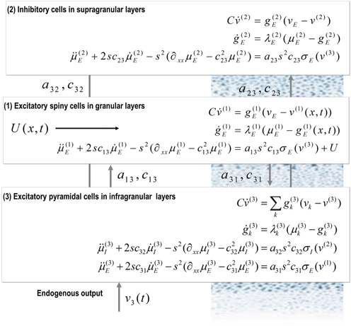

Fig. 3.4
A conductance-based neural field model. This schematic summarizes the equations of motion or state equations that specify a conductance based neural field model of a single source. This model contains three populations, each associated with a specific cortical layer. These equations describe changes in expected neuronal states (e.g., voltage or depolarization) that subtend observed local field potentials or EEG signals. These changes occur as a result of propagating presynaptic input through synaptic dynamics. Mean firing rates within each layer are then transformed through a nonlinear (sigmoid) voltage-firing rate function to provide (presynaptic) inputs to other populations. These inputs are weighted by connection strengths and are gated by the states of synaptic ion channels
This model is a recent addition to conductance based models implemented in the DCM toolbox of the academic freeware Statistical Parametric Mapping (SPM) and has not been yet used for the analysis of empirical data. Here, as a first step, we will consider a single sensor and cortical source driven by white noise input (see also [88]) and illustrate the ability of this model to account for observed evoked responses of the sort recorded with e.g. local field potential electrodes. In particular, we generated synthetic electrophysiological responses by integrating the equations in Fig. 3.4 from their fixed points and characterised the responses to external (excitatory) impulses to spiny stellate cells, in the time domain. Electrophysiological signals (LFP or M/EEG data) were simulated by passing neuronal responses through a lead field that varies with location on the cortical patch. The resulting responses in sensor space (see Figs. 3.5 and 3.6) are given by a mixture of currents flowing in and out of pyramidal cells in Fig. 3.4:
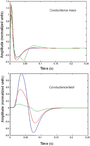
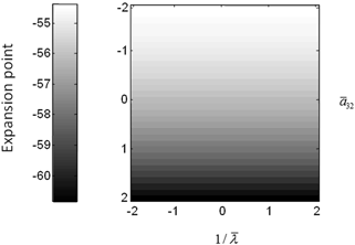

Fig. 3.5
Impulse responses of conductance-based mass and field models. Responses to impulses of different amplitudes for mass (top) and field (bottom) conductance based models. The responses are normalized with respect to the amplitude of each input. The blue lines illustrate responses to small perturbations. The red lines illustrate responses to intermediate sized inputs, where conductance based models show an augmented response, due to their nonlinearity. The green lines show responses for larger inputs, where the saturation effects due to the sigmoid activation function are evident. Nonlinear effects are more pronounced in the field model– with attenuation of the response amplitude, even for intermediate input amplitudes

Fig. 3.6
Conductance mass model mean depolarization. Mean depolarization of the pyramidal population of the conductance neural mass model as a function of parameter changes. This corresponds to the fixed point around which the impulse responses of Fig. 3.5 were computed

(5)
In this equation,  is a vector of coefficients that weight the relative contributions of different populations to the observed signal and
  is the lead field. This depends upon parameters
  and we assume it is a Gaussian function of location—as in previous models of LFP or MEG recordings, see [5]. This equation is analogous to the usual (electromagnetic) gain matrix for equivalent current dipoles. We assume here that these dipoles are created by pyramidal cells whose current is the primary source of an LFP signal. With spatially extended sources (patches), this equation integrates out the dependence on the source locations within a patch and provides a time series for each sensor.
 is a vector of coefficients that weight the relative contributions of different populations to the observed signal and
  is the lead field. This depends upon parameters
  and we assume it is a Gaussian function of location—as in previous models of LFP or MEG recordings, see [5]. This equation is analogous to the usual (electromagnetic) gain matrix for equivalent current dipoles. We assume here that these dipoles are created by pyramidal cells whose current is the primary source of an LFP signal. With spatially extended sources (patches), this equation integrates out the dependence on the source locations within a patch and provides a time series for each sensor.
We modelled a cortical source (approximated with 11 grid points) and used the model equations (see Fig. 3.5) to generate impulse response functions. The parameters of this model are provided in Table 3.2. The results reported below were chosen to illustrate key behaviours in terms of ERPs, following changes in parameter values. We also consider the corresponding result for the mass variant of our field model, that is a simplified Morris-Lecar type model (that neglects fast voltage-dependent conductances) introduced in [24]. This model uses the same equations but assume that all neurons of a population are located at (approximately) the same point.
Table 3.2
Parameters of conductance-based mass and field models. Prior expectation of the conductance-based neural mass and field model parameters
Parameter | Physiological interpretation | Value |
|---|---|---|
 | Leakage conductance | 1 |
 | Amplitude of intrinsic connectivity kernels | (1/10, 1, 1/2, 1)*3/10 (field) 1/2, 1, 1/2, 1 (mass) |
 | Intrinsic connectivity decay constant | 1 (mm−1) |
 | Reversal potential | − 70, 60, − 90 (mV) |
 | Threshold potential | − 40 (mV) |
 | Membrane capacitance | 8 (pFnS−1) |
s | Conduction speed | 3 m/s |
 | Postsynaptic rate constants | 1/4, 1/16 (ms−1) |
 | Radius of cortical patch | 7 (mm) |
The resulting model is based on the Rall and Goldestein equations [101] and is formally related to Ermentrout’s [102] reduction of the model described in [103]. Mass models have often been used to characterize pharmacological manipulations and the action of sedative agents [87, 97, 99, 104–106]. This usually entails assuming that a neurotransmitter manipulation changes a particular parameter, whose effects are quantified using a contribution or structural stability analysis, where structural stability refers to how much the system changes with perturbations to the parameters.
We now focus on generic differences mediated by conductance based field and mass models. To do this, we integrated the corresponding equations for (impulse) inputs of different amplitudes and plotted temporal responses resulting from fixed point perturbations. Linear models are insensitive to the amplitude of the input, in the sense that the impulse responses scale linearly with amplitude. Our interest here was in departures from linearity—such as saturation—that belie the nonlinear aspects of the models. Figure 3.5 shows the responses of the mass and field models to an impulse delivered to stellate cells. Note that these responses have been renormalized with respect to the amplitude of each input. The red (green) curves depict responses to double (ten times) the input reported by the blue curves. We used the same parameters for both models: see Table 3.2.
It can be seen that there are marked differences between the model responses. The top panel depicts the response of the mass model and the lower panel shows the equivalent results for the field model. One can see that large inputs produce substantial sub-additive saturation effects (blue versus green lines in Fig. 3.4): for the mass model, the nonlinearities produce an inverted U relationship between the amplitude of the response, relative to the input. In other words, the form of the input-output amplitude relationship differs quantitatively for the mass (inverted U) and field (decreasing) model (see Fig. 3.5).
The above illustrations of system’s predictions assume that spectral responses result from fixed point perturbations. For conductance models, a change in the parameters changes both the expansion point and the system’s flow (provided the flow is non-zero). Figure 3.5 shows the dependence of the conductance model’s fixed points on parameter perturbations. The model parameterization used here renders the expansion point relatively insensitive to changes in the synaptic time constant. Figure 3.6 shows the results for the conductance mass model; results for its field variant were very similar.
Clinical Applications and Parkinson’s Disease
DCM has contributed to a mechanistic understanding of brain function and drug mechanisms and could serve as an important diagnostic tool for diseases linked to abnormalities in connectivity and synaptic plasticity, like schizophrenia [107–109], Parkinson’s [110–114], consciousness and drug effects [115–119] and epilepsy [120–128]. For some other important clinical applications of DCM the reader is referred to [129–135].
In the following, we discuss an application to Parkinson’s disease focusing on pathological alterations of beta oscillations in Parkinsonian patients and evidence for an abnormal increase in the gain of the cortical drive to STN and the STN-GPe coupling [111]. In line with a previous study in the rat model [110], we used a DCM for steady state responses (SSR) to predict observed spectral densities [4]. The dynamics of these sources is specified by a set of first-order differential equations [110]. The ensemble firing of one population drives the average membrane potential of others through either glutamate (which produces postsynaptic depolarisation) or GABA (hyperpolarisation) as a neurotransmitter. These effects are mediated by a postsynaptic (alpha) kernel that is either positive or negative. The (excitatory or inhibitory) influence of one subpopulation on another is parameterised by extrinsic effective connectivity (between sources) or intrinsic connectivity (within sources). Effective connectivity is modelled as a gain factor that couples discharge rates in one subpopulation to depolarisation in another.
The validity of the approach used here (DCM for SSR) has been addressed previously ([4, 136]). These studies established that both the form of the model and its key parameters can be recovered in terms of conditional probability densities. We first used synthetic datasets that included noisy data and tested for face validity and indentifiability. We ensured the inversion scheme was able to recover veridical estimates and that model comparison using the log-evidence was able to identify the correct model. We also established physiological validity of the model, using empirical LFP data. For more details, we refer the interested reader to ([4, 136]).
In the application of DCM to Parkinsonian circuits considered here, it is not possible to sample more than a few sites in patients. This calls for an assessment of robustness of the spectral DCM in face of ‘hidden’ neuronal areas. To address this, we generated synthetic data from a model where the underlying network of regions was known, and used this dataset to evaluate the model evidence of a family of DCM models that differed in architecture and, more significantly, in hidden neuronal area number. We also evaluated the precision of the connectivity parameter estimates for each model by permuting the amount of available data in each network. These results showed that DCM was able to identify the correct model and recover the true parameter values reliably in settings with different levels of observation noise.
Stay updated, free articles. Join our Telegram channel

Full access? Get Clinical Tree


