Toward Networks from Spikes

to indicate the set of all event pairs wherein an event on neuron A precedes an event on neuron B by time ${t_i}$ . These sets are sometimes referred to as frequent episodes, a term taken from the literature on data mining of event streams in general [15]. We are looking for repeating patterns in the multi-electrode event stream.

If a spatiotemporal pattern of spike events of length M is repeated N times in a single trial, how can we decide how to look for it in a large multi-neuron spike train? With the polychronous group model as our guide we focus our search on instances of fixed time differences between sets of events on electrode pairs. The schematic raster plot of a subset of the events in a trial (Fig. 10.1) shows why this might be appealing in this context. Imagine a set of events that are causally connected as in a polychronous group—initiating the firing sequence by exciting a small number of neurons leads to activation of the neurons in the group according to the pattern shown in Fig. 10.1. The pattern involves three electrodes (coded in the diagram as red, blue, and green) and includes 11 events in each instance. The pattern occurs twice in this example. 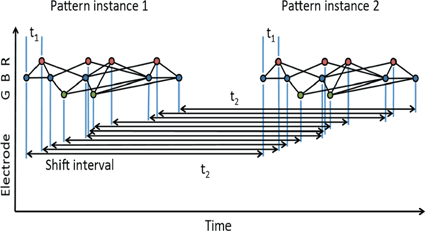Note that the time delay for corresponding events is constant ( ${t_2}$ in this example), which we denote as the shift interval. We denote the collection of events in these two instances together with the shift interval as a shift set. We refer to the number of events in an instance of this firing pattern as the shift set length.

Fig. 10.1

A shift set. This example of repeated firing patterns illustrates the repeating pairwise intervals that they induce. Color of node (red, blue, green) corresponds to electrode (neuron) label on the left (R, B, G). Lines connecting events indicate causal connection, possibly synaptic connection. This diagram follows Izhikevich [11]

Using the color coding of the neuronal associations, the sequence reads: B-R-B-G-B-R-G-R-B-R-B. We can characterize two classes of repeated event pairs from this repeated pattern as follows.

Intra-pattern intervals: Taking the first two events in the sequence as an example, episodes $B[{t_1}]R$ will be found in the event stream as many times as the pattern is found, that is, N times. For this class of frequent episode, there are $\left(\begin{array}{l}M\\2\end{array} \right) = \frac{{M(M - 1)}}{2}$ pairs of neurons to consider within the pattern. Each of these pairs will contribute N instances of an interval to the spectrum of pairwise event time differences. That is, there will be $\left(\begin{array}{l}M\\2\end{array} \right)$ peaks that are N instances tall. The total number of pairs that will contribute to the spectrum is $\left(\begin{array}{l}M\\2\end{array} \right) \times N = \frac{{NM(M - 1)}}{2}$ , a measure of the overall impact of this feature on the spectrum of intervals.

Inter-pattern intervals: Likewise, considering the delay between start of each pattern instance, ${t_2}$ , we note that episodes $X[{t_2}]X$ , where X is any one of the recorded neurons, will be found as many times as there are events in the pattern. We call this list of event pairs a shift set. For N instances of the pattern, there are $\left(\begin{array}{l}N\\2\end{array} \right)$ pattern instance pairs. Each of these pattern pairs, leading to a shift set, will contribute M instances of the interval representing the offset between the onset of each instance. There will be $\left(\begin{array}{l}N\\2\end{array} \right)$ peaks that are M tall. The total number of pairs participating is $\left(\begin{array}{l}N\\2\end{array} \right) \times M = \frac{{MN(N - 1)}}{2}$ . A key distinguishing factor between the intra- and inter-pattern intervals is that the latter collects pairs where the participating neurons are the same in each pair, as in: $B[{t_2}]B,R[{t_2}]R,B[{t_2}]B,G[{t_2}]G,B[{t_2}]B,R[{t_2}]R,$ etc.

One can add background noise and ask how the two perspectives will compare to one another. Conspicuous peaks in the spectrum will indicate either the presence of long patterns, where the number of event pairs in the peak will correlate to the length of the pattern, M; or, high repetition count of smaller patterns, large N. Interpreting such peaks would require different analysis approaches depending on which of these cases holds true.

Note that in addition to the two repeating sets of pairwise delays just described, the existence of an MN pattern in the spike train also contributes a great number of pairwise delays that derive from events taken from different instances of the pattern, but not the special subset of those comprising the shift sets. An example: the delay between the first event in one instance of the pattern, and the second event in another instance. Given the supposed N instances of the M-length pattern, there will be $\left(\begin{array}{l}MN\\2\end{array} \right)$ total distinct event pairs that might contribute to the computed spectrum of delays. This is a number in excess of the two much smaller subsets computed above. For example, with

there will be 450 intra-pattern intervals and another 450 inter-pattern intervals. Compare this to 4050 delays that are neither inter- or intra-pattern. These will in general contribute to the noise floor against which we are trying to detect the patterns.

Distribution of Event Pair Delays

Spike rasters were obtained from a band filtered (300–1500 Hz) version of the broadband signals (Fig. 10.2). A typical raster plot from one trial is shown in Fig. 10.3a. Signals from nine electrodes were selected from the region of the MEA that was most active. Figure 10.3b depicts the same data plotted after shuffling the intervals in the event stream. This procedure preserves the overall number of events on each electrode, as well as the firing sequence across electrodes. Much of the bursting structure of the time series is preserved, but even by eye it is apparent that the distribution on bursting time scales has been affected by the interval shuffling procedure. Figure 10.3c and 10.3d show the corresponding fine-temporal distribution of spike events in three detailed views of typical bursts.

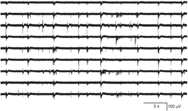
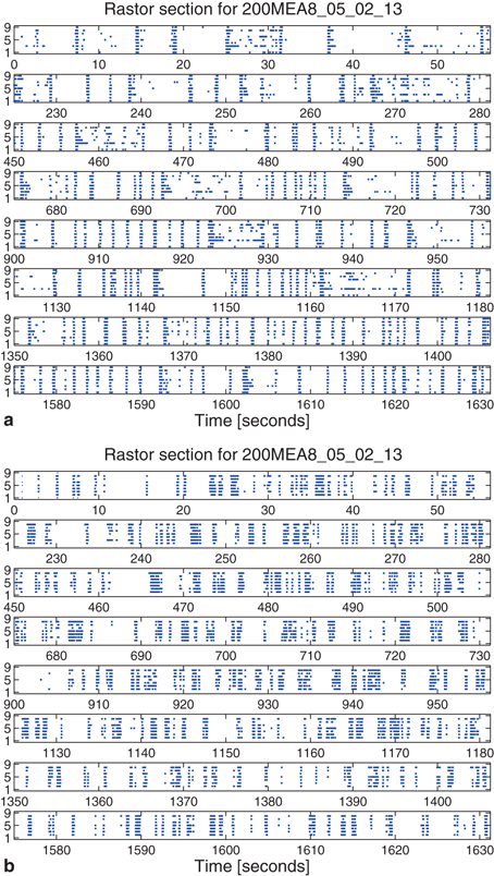
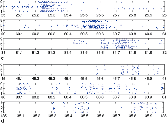
Fig. 10.2

A representative subset of broadband signals (bandwidth 1–3000 Hz) recorded with a multielectrode array setup. The activity patterns depict low frequency waveforms and synchronous as well as asynchronous multi-unit spiking activity

Fig. 10.3

Raster plot of spike train from a multi-electrode array recording: (a) typical raster of nine very active channels from a 30-min recording, and (b) the corresponding surrogate data generated by interval shuffling. They include eight slices of 56 s taken at the beginning of each 225 s segment of the 1800 s recording to show behavior across the entire recording. Also shown are three detailed examples of 1 s rasters of typical bursts showing observed spikes (c) and the surrogate data (d)

The event data from a trial can be described in terms of an event list, ${E_i}$ , which is a set of tuples $\{{T_i},{N_i}\}$ with ${T_i}$ the time of the ${i^{th}}$ event, and ${N_i}$ the channel number of the MEA. We compute all of the intervals between events in the list, giving a list ${I_{ij}}$ of tuples $\{({T_i} - {T_j}),{N_i},{N_j}\}$ such that $$$({T_i} - {T_j})> 0$$ ” src=”/wp-content/uploads/2016/12/A319630_1_En_10_Chapter_IEq23.gif”></SPAN>. We define a shift set as the set of all intervals <SPAN id=IEq24 class=InlineEquation><IMG alt=$ such that $({T_i} - {T_j}) = {T_s}$ , some constant shift interval, and ${N_i} = {N_j}$ for each of the intervals in the set. This notation provides a little more detail than our earlier characterization in terms of episodes, $X[{t_i}]X$ .

Note that the neuron set associated with the shift set is only a candidate as a polychronous group. This is because we don’t have any information about the causal relationships between the events in the set. If a polychronous group is represented in the spike train by firing at least twice, then there will be a shift set that captures it’s signature, perhaps many shift sets— $\left(\begin{array}{l}M\\2\end{array} \right)$ if the group fires M times in the recording. The shift set is a list of neurons that fired two times separated by a specific delay time. A subset of that ordered list of neurons might belong to a polychronous group: (1) there may be neurons represented in the shift set that are serendipitously there because they happened to fire with the delay in question; (2) since we are not sampling all neurons, there may be more neurons in the full polychronous group that we are not even recording.

Given this definition, it is now possible to find all shift sets by sorting and filtering the aggregate interval list. For each value of ${T_s}$ , there may be more than one entry in the interval list for which the above conditions (namely, ${I_{ij}}$ such that $({T_i} - {T_j}) = {T_s}$ , some constant shift interval, and ${N_i} = {N_j}$ ). If so, we have a shift set whose length is given by the number of entries meeting this condition.

The distribution of shift set delays of the data shown in Fig. 10.4 has a number of important features. For delays longer than 1.5 s (middle of the plot), and in fact out to 80 s where the analysis ends (not shown), the observed (black dots) and surrogate data (blue line) are remarkably similar, fluctuating around a constant number of event pairs (around 350 for this 1.6 ms binned data) sharing the delay value. The delay range between approximately 850 ms and 1.5 s appears to be a transition zone. Below 850 ms we see that the principal difference in the distributions is evident. The observed distribution is much more peaked toward short delays than the shuffled surrogate data, as is evident in the 1 s burst details shown in Fig. 10.3c and 10.3d.

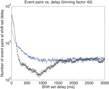
Fig. 10.4

The distribution of delays between event pairs on the same neuron, X[t]X, up to delay t = 3 s. Observed data (black dots) and surrogate data (blue line) continue to overlap at a constant occurrence level out to 80 s, the maximum delay considered in the analysis

Distribution of Shift Set Lengths

The distribution of shift set lengths is shown in Fig. 10.5. In each of the plots, the measured data is shown with points while the surrogate data is shown as a line. Binning factors of 1, 4, and 20 are plotted from left to right.

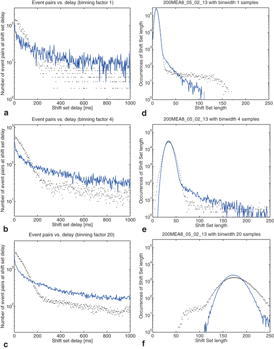
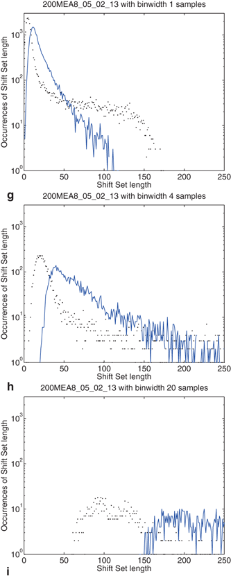
Fig. 10.5

Effects of binning on distributions drawn from the observed data and compared to surrogate data. Binning factors of 1, 4, and 20 are shown from top to bottom, corresponding to bin widths of 0.04, 0.16, and 0.8 ms. (a–c) The distribution of delays (as in Fig. 10.4) between event pairs up to 1 s; (d–f) the distribution of shift set lengths taking all delays up to 80 s; (g–i) includes only delays up to 850 ms

There are several noteworthy observations we would make about the distribution of shift set lengths and its relationship to the distribution of event pair delays (between a single neuron). Consider first the surrogate data (blue line) in all plots. Looking at the distribution of shift set lengths (Fig. 10.5d, 10.5e and 10.5f), it appears to be comprised of two component subpopulations. Most of the expected shift set lengths are contained in a large peak that moves to the right, becoming shorter and wider with increasing binning factor. As noted in the previous section, the distribution of shift set delays asymptote to a constant value (Figs. 10.4 and 10.5a, 10.5b and 10.5c). The large peak in the length distribution contains all of the shift set delays from 1.5 s out to 80 s (we didn’t analyze delays longer than this). The peak is centered on the asymptotic constant, and has a width set by the fluctuations in shift set length around this constant.

Only gold members can continue reading. Log In or Register to continue