Fig. 5.1
Schematic of “working brain” model, showing structures involved in corticothalamic generation of EEGs and the brainstem-hypothalamus ascending arousal system (see section “Arousal State Modeling” for abbreviations), with some of their main inputs, connections, and feedbacks shown by arrows. Adapted from Ref. [82]
Modeling
In this section we briefly review the key corticothalamic and arousal-system sectors of our model, parameter calibration, and links between the two sectors. More detailed discussion and further generalizations can be found elsewhere [63, 64, 68, 70, 72]. We note that other variants of most individual aspects of the model exist in the literature, but that detailed discussion of these variants is beyond the scope of the present chapter, where our aim is to unite the sectors as shown in Fig. 5.1.
General Neural-Field Modeling
The brain contains multiple populations of neurons, which we distinguish by a subscript  that designates both the structure in which a given population lies (e.g., a particular nucleus) and the type of neuron (e.g., interneuron, pyramidal cell). We average their properties over scales of ~ 0.1 mm and seek equations for the resulting mean-field quantities.
that designates both the structure in which a given population lies (e.g., a particular nucleus) and the type of neuron (e.g., interneuron, pyramidal cell). We average their properties over scales of ~ 0.1 mm and seek equations for the resulting mean-field quantities.The mean soma potential  (measured relative to rest here) is approximated as the sum of contributions
  arriving as a result of activity at each type of (mainly) dendritic synapse
  , where
  denotes both the population and neurotransmitter type,
  is the spatial coordinate, and
  the time. This gives
(measured relative to rest here) is approximated as the sum of contributions arriving as a result of activity at each type of (mainly) dendritic synapse , where denotes both the population and neurotransmitter type, is the spatial coordinate, and the time. This gives
(5.1)
The potential  is generated when synaptic inputs from afferent neurons
  are temporally low-pass filtered and smeared out in time as a result of receptor dynamics and passage through the dendrites of neurons
  (i.e., by dynamics of ion channels, membranes, etc.). It approximately obeys the differential equation [69, 79, 72, 75]
is generated when synaptic inputs from afferent neurons are temporally low-pass filtered and smeared out in time as a result of receptor dynamics and passage through the dendrites of neurons (i.e., by dynamics of ion channels, membranes, etc.). It approximately obeys the differential equation [69, 79, 72, 75]
(5.2)
(5.3)
where  and
and  are the characteristic rise and decay times of the potential change due to an impulse at a dendritic synapse. The right of Eq. (5.2) describes the influence of the firing rates
  from neuronal populations
  , in general delayed by a time
  due to discrete anatomical separations between different structures. The quantity
  is the mean number of synapses to neurons of type
  from type
  , and
, and  is the time-integrated response in neurons of type
  to a unit signal from neurons of type
  , implicitly weighted by the neurotransmitter release probability. In the present chapter we treat the
  as constants and ignore their dynamics, which can be driven by neuromodulators, firing rate, and other effects; however, such dynamics can be incorporated straightforwardly [e.g., [13]].
and are the characteristic rise and decay times of the potential change due to an impulse at a dendritic synapse. The right of Eq. (5.2) describes the influence of the firing rates from neuronal populations , in general delayed by a time due to discrete anatomical separations between different structures. The quantity is the mean number of synapses to neurons of type from type , and is the time-integrated response in neurons of type to a unit signal from neurons of type , implicitly weighted by the neurotransmitter release probability. In the present chapter we treat the as constants and ignore their dynamics, which can be driven by neuromodulators, firing rate, and other effects; however, such dynamics can be incorporated straightforwardly [e.g., [13]].Action potentials are produced at the axonal hillock when the soma potential  exceeds a threshold, at a rate that rises steeply with
  before leveling off. In a population, this dependence is smeared out by differences in individual neurons and their environments to yield the population-average response function
exceeds a threshold, at a rate that rises steeply with before leveling off. In a population, this dependence is smeared out by differences in individual neurons and their environments to yield the population-average response function![$$ {{Q}_{a}}(\mathbf{r},t)=S[{{V}_{a}}(\mathbf{r},t)], $$](/wp-content/uploads/2016/12/A319630_1_En_5_Chapter_Equ4.gif)
(5.4)


![$$ S[{{V}_{a}}(\mathbf{r},t)]=\frac{{{Q}_{\rm max}}}{1+{\rm exp}\{-[{{V}_{a}}(\mathbf{r},t)-{{\theta }_{a}}]/{\sigma }'\}}, $$](/wp-content/uploads/2016/12/A319630_1_En_5_Chapter_Equ5.gif)
(5.5)
where we assume a common mean neural firing threshold  relative to resting, with
  being its standard deviation (here,
  ,
,  , and
, and  are assumed to be the same in all populations for simplicity). When treating linear perturbations relative to a given state, we make the approximation
relative to resting, with being its standard deviation (here, , , and are assumed to be the same in all populations for simplicity). When treating linear perturbations relative to a given state, we make the approximation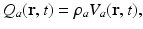
(5.6)
where  and
and  are now perturbations and
  is the derivative of the sigmoid at an assumed steady state of the system in the absence of perturbations (we discuss the existence and stability of such states below).
and are now perturbations and is the derivative of the sigmoid at an assumed steady state of the system in the absence of perturbations (we discuss the existence and stability of such states below).Each neuronal population  in the corticothalamic system produces a field
  of pulses, that travels to other neuronal populations at a velocity
  through axons with a characteristic range
  . This activity spreads out and dissipates if not regenerated. To a good approximation, this type of propagation obeys a damped wave equation [29, 44, 72]:
in the corticothalamic system produces a field of pulses, that travels to other neuronal populations at a velocity through axons with a characteristic range . This activity spreads out and dissipates if not regenerated. To a good approximation, this type of propagation obeys a damped wave equation [29, 44, 72]:![$$ {{D}_{a}}{{\varphi }_{a}}(\mathbf{r},t)=S[{{V}_{a}}(\mathbf{r},t)], $$](/wp-content/uploads/2016/12/A319630_1_En_5_Chapter_Equ7.gif)
(5.7)
(5.8)
where the damping coefficient is  . Eqs. (5.7) and (5.8) yield propagation ranges in good agreement with anatomical results [10]. It is sometimes erroneously claimed that this propagation is an approximation to propagation with delta-function delays of the form
  ; in reality, both mathematical approaches approximate the same physical system. More relevant is the fact that there is actually a range of velocities of propagation in axons [7, 30], which leads to a range of transit times for signals between any two points; however, this effect can be approximated via a corresponding increase in the effective synaptodendritic time constants (thereby spreading the response over a longer interval), which should then be interpreted as axo-synapto-dendritic quantities. More generally, a velocity spread can be introduced into the underlying propagator [8], or an appropriate generalized propagator could be derived.
. Eqs. (5.7) and (5.8) yield propagation ranges in good agreement with anatomical results [10]. It is sometimes erroneously claimed that this propagation is an approximation to propagation with delta-function delays of the form ; in reality, both mathematical approaches approximate the same physical system. More relevant is the fact that there is actually a range of velocities of propagation in axons [7, 30], which leads to a range of transit times for signals between any two points; however, this effect can be approximated via a corresponding increase in the effective synaptodendritic time constants (thereby spreading the response over a longer interval), which should then be interpreted as axo-synapto-dendritic quantities. More generally, a velocity spread can be introduced into the underlying propagator [8], or an appropriate generalized propagator could be derived.Equations (5.1)–(5.5), (5.7), and (5.8) form a closed nonlinear set, which can be solved numerically, or examined analytically in various limits. Once a set of specific neural populations has been chosen, and physiologically realistic values have been assigned to their parameters, these equations can be used to make predictions of neural activity. These equations govern spatiotemporal dynamics of firing rates; oscillations predicted from them are emergent changes of the average rate of spiking, whose frequencies do not usually equal the spiking frequency itself.
Corticothalamic System
Much work has been done on applications of our neural field theory to the corticothalamic system, which is the first sector of the combined model of Fig. 5.1 to be discussed. This work has also included extensive verification and validation of the predictions against experiment, as discussed in the next section.
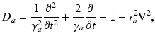
Figure 5.2 shows the large-scale structures and connectivities incorporated, including the thalamic reticular nucleus  , which inhibits relay (or specific) nuclei
  , and is lumped here with the perigeniculate nucleus, which has an analogous role [90, 94]. Relay nuclei convey external stimuli
  and pass on corticothalamic feedback. In this section we consider long-range excitatory cortical neurons
  , short-range mainly inhibitory cortical neurons
  , neurons in the reticular nucleus
  , neurons of thalamic relay nuclei
  , and external inputs
  from non-corticothalamic neurons. These populations are discussed further below.
, which inhibits relay (or specific) nuclei , and is lumped here with the perigeniculate nucleus, which has an analogous role [90, 94]. Relay nuclei convey external stimuli and pass on corticothalamic feedback. In this section we consider long-range excitatory cortical neurons , short-range mainly inhibitory cortical neurons , neurons in the reticular nucleus , neurons of thalamic relay nuclei , and external inputs from non-corticothalamic neurons. These populations are discussed further below.


If intracortical connectivities are proportional to the numbers of neurons involved—the random connectivity approximation—then  and
and  for each
  , whence
  and
and  [73, 100]. This lets us concentrate on excitatory quantities, with inhibitory ones derivable from them (we stress that inhibitory effects are still included). The short range of
  neurons and the small size of the thalamic nuclei enables us to assume
  and, hence,
  for
for  for many purposes. The only nonzero discrete delays are
  , where
  is the time for signals to pass from cortex to thalamus and back. We also assume that all the synaptodendritic time constants are equal, for simplicity, and set
  and
and  for all
  and
and  in what follows; this allows us to drop the subscripts
  in Eqs. (5.2) and (5.3) and write
  in place of
  .
.
and for each , whence and [73, 100]. This lets us concentrate on excitatory quantities, with inhibitory ones derivable from them (we stress that inhibitory effects are still included). The short range of neurons and the small size of the thalamic nuclei enables us to assume and, hence, for for many purposes. The only nonzero discrete delays are , where is the time for signals to pass from cortex to thalamus and back. We also assume that all the synaptodendritic time constants are equal, for simplicity, and set and for all and in what follows; this allows us to drop the subscripts in Eqs. (5.2) and (5.3) and write in place of .Including only the connections shown in Fig. 5.2 and making the approximations mentioned above, our nonlinear model has 16 parameters, not all of which appear separately in the linear limit. By defining

(5.9)
these are  . These are sufficient to allow adequate representation of the most important anatomy and physiology, but few enough to yield useful interpretations and to enable reliable calibration of their values by fitting theoretical predictions to data. The parameters are approximately known from experiment [69, 70, 79, 75, 83] leading to the indicative values in Table 5.1. We use only values compatible with physiology. Sensitivities of the model to parameter variations have been explored in general [75] and in connection with variations between arousal states [76], as discussed below.
. These are sufficient to allow adequate representation of the most important anatomy and physiology, but few enough to yield useful interpretations and to enable reliable calibration of their values by fitting theoretical predictions to data. The parameters are approximately known from experiment [69, 70, 79, 75, 83] leading to the indicative values in Table 5.1. We use only values compatible with physiology. Sensitivities of the model to parameter variations have been explored in general [75] and in connection with variations between arousal states [76], as discussed below.Parameter | Description | Eyes-open | Spindle | Unit |
|---|---|---|---|---|
 | Maximum firing rate | 340 | 340 | s−1 |
 | Axonal velocity | 10 | 10 | ms−1 |
 | Axonal range | 86 | 86 | mm |
 | Firing threshold | 12.9 | 12.9 | mV |
 | Threshold spread | 3.8 | 3.8 | mV |
 | Cortical damping rate | 116 | 116 | s−1 |
 | Corticothalamic loop delay | 85 | 85 | ms |
 | Synaptodendritic decay time | 12 | 22 | ms |
 | Synaptodendritic rise time | 1.3 | 5.4 | ms |
 | Connection strength (  from from  ) ) | 7.85 | 3.06 | mV s |
 | Connection strength (  from from  ) ) | 9.88 | 3.24 | mV s |
 | Connection strength (  from from  ) ) | 0.90 | 0.92 | mV s |
 | Connection strength (  from from  ) ) | 2.68 | 4.73 | mV s |
 | Connection strength (  from from  ) ) | 1.31 | 1.95 | mV s |
 | Connection strength (  from from  ) ) | 6.60 | 2.70 | mV s |
 | Connection strength (  from from  ) ) | 0.21 | 0.26 | mV s |
 | Connection strength (  from from  ) ) | 0.06 | 2.88 | mV s |
 | Steady state firing rate (  ) ) | 5.2 | 8.5 | s−1 |
 | Steady state firing rate (  ) ) | 16.3 | 27.8 | s−1 |
 | Steady state firing rate (  ) ) | 8.4 | 0.5 | s−1 |
 | Steady state firing rate (  ) ) | 1 | 1 | s−1 |
An important implication of the parameters above is that the corticothalamic loop delay  places any oscillations that involve this loop at frequencies of order 10 Hz. This means that inclusion of the thalamus and the dynamics of these loops is essential to understand phenomena at frequencies below ~20 Hz. At frequencies << 10 Hz it is sufficient to include a static corticothalamic feedback strength, and at frequencies >> 10 Hz the corticothalamic feedback is too slow and too attenuated by low-pass effects to influence the dynamics strongly.
places any oscillations that involve this loop at frequencies of order 10 Hz. This means that inclusion of the thalamus and the dynamics of these loops is essential to understand phenomena at frequencies below ~20 Hz. At frequencies << 10 Hz it is sufficient to include a static corticothalamic feedback strength, and at frequencies >> 10 Hz the corticothalamic feedback is too slow and too attenuated by low-pass effects to influence the dynamics strongly.
(5.10)

(5.11)
(5.12)

(5.13)
whence  and
and  , as asserted above. The right side of each of Eqs (5.10)–(5.13) describes the spatial summation of all afferent activity (including via self-connections) for one neural population, and
  on the left describes temporal dynamics. The short ranges of the axons
  ,
,  , and
, and  imply that the corresponding damping rates are large and that
  for these populations, further implying
and , as asserted above. The right side of each of Eqs (5.10)–(5.13) describes the spatial summation of all afferent activity (including via self-connections) for one neural population, and on the left describes temporal dynamics. The short ranges of the axons , , and imply that the corresponding damping rates are large and that for these populations, further implying
(5.14)


![$$ \left(\frac{1}{\gamma_{e}^{2}}\frac{{{\partial }^{2}}}{\partial {{t}^{2}}}+\frac{2}{{{\gamma }_{e}}}\frac{\partial }{\partial t}+1-r_{e}^{2}{{\nabla }^{2}}\right){{\varphi }_{e}}(\mathbf{r},t)=S[{{V}_{e}}(\mathbf{r},t)], $$](/wp-content/uploads/2016/12/A319630_1_En_5_Chapter_Equ15.gif)
(5.15)
with  . Equations (5.10)–(5.15) describe our corticothalamic model. The neural mass limit correponds to
  , when all delays within populations are negligible compared to the timescales of the phenomena of interest.
. Equations (5.10)–(5.15) describe our corticothalamic model. The neural mass limit correponds to , when all delays within populations are negligible compared to the timescales of the phenomena of interest.Once neural activity has been predicted from stimuli, one must relate it to measurements to interpret experimental results. The limited spatiotemporal resolution of such measurements often provides an additional justification for the use of mean-field modeling, since finer structure is not resolvable. The quantity  dominates in determining both EEG and fMRI signals—the former because of the dominance and highly aligned dipoles of pyramidal cells, the latter because of pyramidal cells’ predominance in cortical metabolic load. In both cases, it is the synaptic dynamics that predominate in determining the measured signals, so
  (not
(not  ) is the relevant variable. These points have been discussed in detail elsewhere [78, 71, 45, 74, 30].
dominates in determining both EEG and fMRI signals—the former because of the dominance and highly aligned dipoles of pyramidal cells, the latter because of pyramidal cells’ predominance in cortical metabolic load. In both cases, it is the synaptic dynamics that predominate in determining the measured signals, so (not ) is the relevant variable. These points have been discussed in detail elsewhere [78, 71, 45, 74, 30].Arousal State Modeling
Transitions between wake and sleep states are primarily governed by the nuclei of the ascending arousal system (AAS) of the brainstem and hypothalamus, that project diffusely to the corticothalamic system, receive inputs from the suprachiasmatic nucleus (SCN) and elsewhere, and interact with sleep-promoting nuclei [86, 85]. A full description of sleep–wake transitions and their EEG correlates requires an integrated model of both the ascending arousal system and the corticothalamic system, including their mutual interactions. This section briefly describes how the nuclei of the AAS are modeled using the same methods as above [82].
The most important nuclei to model in the AAS are well established from physiology, and are shown in Fig. 5.1. These include the wake-promoting monoaminergic (MA) group and the sleep-promoting ventrolateral preoptic nucleus (VLPO), which inhibit one another, resulting in flip-flop dynamics if they interact strongly—only one is active at a time, and suppresses the other [84, 86, 85] to form the sleep-wake switch. In wake the MA is dominant, and in sleep the VLPO is dominant. State transitions are driven by inputs to the sleep-wake switch, including the circadian drive  from the SCN and the homeostatic sleep drive
  from buildup of metabolites (likely including adenosine, Ad, related compounds, or their byproducts) in wake and their clearance in sleep [55, 38, 101]. Cholinergic (ACh) and orexinergic (Orx, not shown in Fig. 5.1) inputs to the MA group are also present [48, 86, 85].
from the SCN and the homeostatic sleep drive from buildup of metabolites (likely including adenosine, Ad, related compounds, or their byproducts) in wake and their clearance in sleep [55, 38, 101]. Cholinergic (ACh) and orexinergic (Orx, not shown in Fig. 5.1) inputs to the MA group are also present [48, 86, 85].Most models of human sleep have been either nonmathematical (e.g., based on sleep diaries) or abstract (mathematical, but not derived directly from physiology). The widely known two-process model is of the latter form, and includes circadian and homeostatic influences [15, 3]. Recent advances in sleep neurophysiology have enabled development of physiologically based models [51, 97, 16, 56, 62, 9]; here we use neural mass theory (NMT) to model the dynamics of the AAS nuclei.
Phillips and Robinson [51] argued that (i) since the system spends little time in transitions, the generation rate of  can be approximated as having two values, one for wake and one for sleep, (ii) the clearance rate of
  is assumed to be proportional to
  with a characteristic time scale
  , and (iii) the production rate of
  is
is  , where
  is a constant and
  serves as a proxy for arousal state. These steps yield equations for
  and the mean soma voltages
  in the MA group (
 ) and VLPO (
 ):
):
can be approximated as having two values, one for wake and one for sleep, (ii) the clearance rate of is assumed to be proportional to with a characteristic time scale , and (iii) the production rate of is , where is a constant and serves as a proxy for arousal state. These steps yield equations for and the mean soma voltages in the MA group () and VLPO ():
(5.16)
(5.17)
(5.18)

(5.19)
(5.20)
where the time constants  and
and  of the responses have been assumed equal to a common value
  [these replace
  in Eq. (5.3), with
  formally],
  is the somnogen clearance time,
  denotes VLPO,
  denotes MA, the
  ,
,  , and
, and  have the same meanings as in previous sections,
  gives the proportionality between monoaminergic activity and somnogen generation rate.
and of the responses have been assumed equal to a common value [these replace in Eq. (5.3), with formally], is the somnogen clearance time, denotes VLPO, denotes MA, the , , and have the same meanings as in previous sections, gives the proportionality between monoaminergic activity and somnogen generation rate.The total sleep drive  to the VLPO comprises
  and
and  , where
  can be interpreted as the SCN firing rate and
  is a firing rate change due to somnogenic effects; in both cases only the terms
  and
and  influence
  . The
. The  is a constant baseline level for the total sleep drive. When circadian entrainment to the natural light-dark cycle can be assumed, one has
to the VLPO comprises and , where can be interpreted as the SCN firing rate and is a firing rate change due to somnogenic effects; in both cases only the terms and influence . The is a constant baseline level for the total sleep drive. When circadian entrainment to the natural light-dark cycle can be assumed, one has
(5.21)
where  is the angular rate of Earth’s rotation, and the amplitude of
  is absorbed into
  .
.
is the angular rate of Earth’s rotation, and the amplitude of is absorbed into .In other cases, such as jetlag and shiftwork,  is modeled using the human circadian pacemaker model of St Hilaire et al. [96], which is the most recent version of the well-known model of the human circadian oscillator by Kronauer et al. [34]. The model includes (i) a light processing component, (ii) a component for the effects of non-photic stimuli, and (iii) a van der Pol oscillator component.
is modeled using the human circadian pacemaker model of St Hilaire et al. [96], which is the most recent version of the well-known model of the human circadian oscillator by Kronauer et al. [34]. The model includes (i) a light processing component, (ii) a component for the effects of non-photic stimuli, and (iii) a van der Pol oscillator component.In light processing, retinal photoreceptors are converted from ready to activated state by photons at a rate  , dependent on light intensity
  :
:
, dependent on light intensity :
(5.22)
where  ,
,  , and
, and  are constants used to adjust the model dynamics to experimental data. Activated photoreceptors are converted back to ready at a constant rate
  . Thus the fraction
  of activated photoreceptors follows
, , and are constants used to adjust the model dynamics to experimental data. Activated photoreceptors are converted back to ready at a constant rate . Thus the fraction of activated photoreceptors follows
(5.23)
The resultant photic drive  is proportional to the rate
  and the fraction of photoreceptors that can be activated
  :
:
is proportional to the rate and the fraction of photoreceptors that can be activated :
(5.24)
where  and
and  are constants adjusted to fit experimental data [96], and
  and
and  are the circadian variables of the oscillator. The term
  accounts for the experimentally observed phase-dependent sensitivity of the circadian pacemaker to light.
and are constants adjusted to fit experimental data [96], and and are the circadian variables of the oscillator. The term accounts for the experimentally observed phase-dependent sensitivity of the circadian pacemaker to light.The non-photic effects, such as meals and locomotion, on the circadian oscillator are modeled as increased stimulation during wake hours:
![$$ {{N}_{s}}=\rho \left(\frac{1}{3}-s \right)[1-\text{t}{\rm anh}(10x) ], $$](/wp-content/uploads/2016/12/A319630_1_En_5_Chapter_Equ25.gif)
(5.25)
where  is a constant reflecting strength of the non-photic stimulation, and
  equals 1 during wakefulness and 0 during sleep, providing for state-dependency. The factor in the square brackets accounts for stronger nonphotic effects near the minimum of core body temperature [96].
is a constant reflecting strength of the non-photic stimulation, and equals 1 during wakefulness and 0 during sleep, providing for state-dependency. The factor in the square brackets accounts for stronger nonphotic effects near the minimum of core body temperature [96].The circadian oscillator thus follows
![$$ \frac{dx}{dt}=\Omega \left[{{x}_{c}}+\gamma \left(\frac{1}{3}x+\frac{4}{3}{{x}^{3}}-\frac{256}{105}{{x}^{7}}\right)+B+{{N}_{s}}\right], $$](/wp-content/uploads/2016/12/A319630_1_En_5_Chapter_Equ26.gif)
(5.26)
![$$ \frac{d{{x}_{c}}}{dt}=\Omega \left[qB{{x}_{c}}-x\left\{{{\left(\frac{\delta }{{{\tau }_{c}}}\right)}^{2}}+kB \right\} \right], $$](/wp-content/uploads/2016/12/A319630_1_En_5_Chapter_Equ27.gif)
(5.27)
where  is the pacemaker activity,
  is a complementary variable,
  is an intrinsic circadian period,
  is the stiffness of the oscillator,
  and
and  determine strength of the photic drive
  ,
,  is a correction factor that ensures the correct intrinsic circadian period, and
  is positive for diurnal animals [34, 28]. The numerical coefficients in Eqs. (5.26) and (5.27) were chosen to achieve unit amplitude of the limit cycle.
is the pacemaker activity, is a complementary variable, is an intrinsic circadian period, is the stiffness of the oscillator, and determine strength of the photic drive , is a correction factor that ensures the correct intrinsic circadian period, and is positive for diurnal animals [34, 28]. The numerical coefficients in Eqs. (5.26) and (5.27) were chosen to achieve unit amplitude of the limit cycle.Core body temperature (CBT) demonstrates circadian fluctuations and timing of CBT minimum is often used as a marker of circadian phase. In entrained individuals it typically appears about 2 h before awakening, and is calculated as:
(5.28)
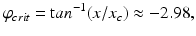
(5.29)
where  h is a constant and
  is a phase difference between the circadian variables
  and
and  given in radians.
h is a constant and is a phase difference between the circadian variables and given in radians.Connections between the AAS and the circadian oscillator systems are reciprocal: (i) the circadian variable  has an effect on the VLPO, as described in Eq. (5.20), and (ii) the AAS system has an effect on
  by reducing (or setting to zero lux) the light input
  during sleep.
has an effect on the VLPO, as described in Eq. (5.20), and (ii) the AAS system has an effect on by reducing (or setting to zero lux) the light input during sleep.The parameters in the above model have the nominal values in Table 5.2, determined by physiological constraints from the literature and comparison with a restricted set of experiments on normal sleep, sleep deprivation, and the effects of light on circadian phase [51, 52, 96, 34, 28]. The theory then predicts phenomena in regimes outside those of the calibration experiments, with only slight adjustments to account for individual state and trait differences—these adjustments can be compared with what is expected from independent physiological analyses; e.g., a long circadian period  should be associated with the evening (“night owl”) chronotype, while short
  should be associated with morning type [54].
should be associated with the evening (“night owl”) chronotype, while short should be associated with morning type [54].Table 5.2
Parameter values of the AAS model and their units. The sigmoid parameters carry an extra prime to indicate that they can differ from the cortical values in Table 5.1
AAS | Circadian pacemaker | ||||
|---|---|---|---|---|---|
Quantity | Nominal | Unit | Quantity | Nominal | Unit |
 | 100 | s−1 |  |  | s−1 |
 | 10 | mV |  | 1/3 | – |
 | 3 | mV |  | 0.55 | – |
 | − 2.1 | mV s |  |  | s |
 Related posts: Introduction
Epileptogenic Networks: Applying Network Analysis Techniques to Human Seizure Activity
Computational Modeling of Neuronal Dysfunction at Molecular Level Validates the Role of Single Neurons in Circuit Functions in Cerebellum Granular Layer
Toward Networks from Spikes
DCM, Conductance Based Models and Clinical Applications
Computational Models of Closed–Loop Deep Brain Stimulation Introduction
Epileptogenic Networks: Applying Network Analysis Techniques to Human Seizure Activity
Computational Modeling of Neuronal Dysfunction at Molecular Level Validates the Role of Single Neurons in Circuit Functions in Cerebellum Granular Layer
Toward Networks from Spikes
DCM, Conductance Based Models and Clinical Applications
Computational Models of Closed–Loop Deep Brain Stimulation
Stay updated, free articles. Join our Telegram channel
Full access? Get Clinical Tree
 Get Clinical Tree app for offline access

| |||||