Computational Anatomy in Alzheimer’s Disease Alex D. Leow, Liana G. Apostolova and Paul M. Thompson

INTRODUCTION

Alzheimer’s disease (AD) is the most common form of dementia, afflicting over 24 million people worldwide. In early AD, short-term memory function is typically among the first to be impaired, followed by a progressive decline in other cognitive functions along with emotional/behavioural disturbances. At present, there is no cure for AD, whose natural course is insidious yet gradually debilitating, and is typically fatal at its most advanced stage, usually due to medical complications. In recent years, scientific interest has also focused on mild cognitive impairment (MCI), a pre-dementia stage that carries a four- to six-fold increased risk of future diagnosis of dementia, relative to the general population^1-3.

Many investigators have used MRI and PET imaging to measure longitudinal progression of brain changes in normal aging, MCI and AD, with varying results. As drug candidates that might slow the progression of Alzheimer’s pathology began to be developed, the need for robust and sensitive imaging methods to quantify progression of Alzheimer’s disease has become increasingly important. As a result, we are starting to see large collaborative multicentre imaging studies on Alzheimer’s disease. For example, the National Institute of Aging and pharmaceutical industry funded the Alzheimer’s Disease Neuroimaging Initiative⁴⁵ (ADNI), with the goal of developing improved methods based on imaging and other biomarkers, for AD treatment trials.

Major advances are occurring in scanning techniques and in image analysis, making it easier to track disease progression with greater power. In studies of hundreds of subjects scanned over time, databases of images can now be combined to visualize the disease trajectory, showing the spread of cortical atrophy, impaired metabolism, and even plaque and tangle accumulation. Ultra-high-field MRI reveals early changes in specific hippocampal subfields^4,5, and new PET ligands are emerging to visualize plaque and tangle pathology^6-9.

In this chapter, we review several strategies of computational anatomy in mapping brain deficits in AD and early dementia. These strategies include cortical thickness mapping, tensor-based mor- phometry (TBM) and hippocampal surface modelling. Mathematical concepts from surface modelling, non-linear three-dimensional volume registration, fluid mechanics and multivariate statistics are used across subjects for group and interval comparisons. They can be exploited to distinguish diseases from normal variations in brain structure, and help yield insights into the dynamics of AD and MCI.

COMPUTATIONAL ANATOMY

Computational anatomy is a general term covering a broad class of mathematical methods that model anatomical structures in images as three-dimensional curves, surfaces and volumes, and combine them across subjects to create statistical maps of brain structural differences.

Cortical Thickness Mapping

In this approach, in order to precisely quantify the amount of tissue loss, overall grey and white matter volumes can be computed from brain MRI scans. Tissue classification methods can assign each image voxel to a specific tissue class. If grey matter maps from many subjects are aligned to a standard three-dimensional digital brain atlas, on which lobar subdivisions have been labelled, regional statistics for subdivisions can be derived. These region-of-interest measures, in conjunction with manual tracings of the hippocampus and other sub- cortical structures, have been the mainstay of morphometric analysis for nearly two decades.

One approach for cortical thickness mapping is presented in Figure 46.1, which shows a computational pipeline for processing MRI scans as described by Thompson et al.¹⁰. For each scan, a three-dimensional map is first computed quantifying the distance of cortical grey matter voxels to the grey/white matter interface. Thickness values are calculated from the inner cortical surface to the outer cortical surface, and are plotted at each point on a cortical surface model extracted from the scan. To combine thickness data across subjects (Figure 46.1, second row), a spherical coordinate system is imposed onto each subject’s cortical surface. This serves as a reference grid so that thickness data can be compared at a given surface-based coordinate across subjects. If sulcal/gyral landmarks are traced onto the cortical models, data from corresponding cortical regions can be averaged across subjects using a technique known as cortical pattern matching¹⁰ (CPM), where the sulcal pattern is digitized and matched across subjects using a flow field in spherical coordinates. By doing so, an average cortical model can be created

Figure 46.1 Flowchart showing an image analysis pipeline (adapted from¹⁰) that can map changes of various neuroanatomical measures in the cortex, such as grey matter atrophy. Cortical thickness profiles, for example, can be averaged across subjects or compared across time. Tissue classification techniques can be used to identify grey and white matter and to produce cortical thickness maps (row 1). The CPM approach can be applied by tracing sulcal landmarks on extracted brain surface models (row 2) that serve as anchors to guide a flow field matching gyral regions across subjects (row 3). Then maps of cortical thickness, or other cortical signals (such as co-registered PET images, shown here), can be fluidly aligned to an average cortical model (row 4). Statistical models are fitted to data from all the subjects at each cortical point. This can assess whether imaging signals are associated with age (bottom row), or other parameters of interest. Effects of ageing on cortical measures – or changes relative to baseline – may be animated as a time-lapse film to reveal the disease trajectory. A full colour version of this figure appears in the colour plate section

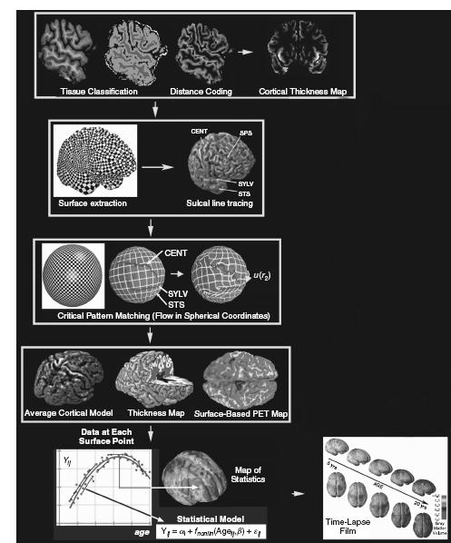
for a group of subjects (such as an AD or MCI population), with well-defined sulcal features in their mean spatial locations (Figure 46.1, fourth row). Moreover, maps of cortical thickness in each individual can be transferred onto this average model while adjusting for the individual gyral pattern differences across subjects. This method allows pixel-by-pixel averaging of values within each delineated region across all subjects, allowing comparisons of patients with controls. Lastly, a statistical model can be fitted to the thickness measures from all subjects at each surface point (Figure 46.1, bottom row). In brain mapping studies, it is common to fit statistical models to data at each location in an image, to assess effects of age, diagnosis or experimental parameters (an approach known as statistical parametric mapping; SPM¹¹). The results are displayed in the form of a three-dimensional map of statistics, and the overall significance of the map can be colour-coded to show the distribution of atrophy¹⁰.

Cortical thickness mapping is related to several simpler but widely used methods. For example, the ‘boundary shift integral’ technique quantifies differences between two successive co-registered 3D MRIs by examining the magnitude of the shifting of grey-white junction¹². Before algorithms became widely available for computing cortical thickness accurately from MRI scans, it was more common to compute a local measure of grey matter volume called ‘grey matter density’ (GMD). This is defined, at each point in an image, as the proportion of tissue segmented as grey matter in a small spherical region (typically of 10-12 mm radius) centred at that point^13,14. GMD and thickness are highly correlated¹⁵, except at the temporal lobe tips, where cortical curvature is high.

Cortical Maps in AD and MCI

Cortical mapping methods have distinguished patterns of atrophy typical of late- versus early-onset AD¹⁶, and different dementia subtypes¹⁷. Sowell et al.¹⁸ applied cortical pattern matching to 176 scans of subjects aged 7 to 87, and compiled trajectories of grey matter thinning, for each cortical point, over the life span. Encouragingly, there was close regional correspondence between the cortical thickness maps created from in vivo MRI and the 1929 postmortem data of von Economo. The cortex does not age in a homogeneous way; each cortical region has a somewhat distinctive trajectory^18,19. A related study by Gogtay et al.²⁰ created a time-lapse map of cortical development from ages 4 to 22, and showed the earliest maturing cortex is least vulnerable to aging and AD.

Apostolova et al.²¹ compared grey matter profiles in 26 amnestic MCI and 31 mild AD subjects, showing strikingly greater atrophy in mild AD (Figure 46.2A), conforming to the pattern of spread of AD pathology observed postmortem through the brain. A related VBM study found significantly greater parietal, anterior and posterior cingulate atrophy in mild to severe AD relative to MCI²³.

In Apostolova et al.²², we also examined the structural correlates of apathy in AD, by applying cortical mapping to 35 AD patients with and without apathy (Figure 46.2B). Apathy severity was associated with cortical grey matter atrophy in bilateral anterior cingulate (Brodmann area BA 24; r = 0.39-0.42, p = 0.01) and left medial frontal cortex (BA 8 and 9; r = 0.4, p < 0.02). A subsequent study found associations between the Boston Naming Test and the animal fluency tests and cortical atrophy in 19 probable AD and 5 multiple-domain amnestic MCI patients who later converted to AD²⁴. The degree of language impairment correlated with cortical atrophy in the left temporal and parietal lobes, especially in the perisylvian language cortices.

Time-Lapse Maps and the Trajectory of AD

The cortical pattern matching approach may be extended to time- varying or functional imaging data. If longitudinal scans are available, a time-lapse movie of disease progression can be created by fitting a trajectory to cortical thickness, or any other imaging parameter, at each cortical point (Figure 46.1, bottom right)²⁵. A movie ‘frame’ can then be written out for each time-point and the series of frames can be animated. An example of this type of dynamic map may be viewed at www.loni.ucla.edu/~thompson/AD_4D/dynamic.xhtml. Here, a time-dependent model was fitted to cortical grey matter density in 14 AD patients and 12 controls scanned longitudinally for 4 years. Maps of the degree of deficits – either as a percentage or as a significance map – show that the cortex is thinner in medial and lateral temporal lobes in early AD and deficits advance anteriorly to engulf the cingulate and frontal cortex.

Figure 46.3 shows two time-points from this animation, showing that cortical atrophy on MRI proceeds in approximately the same anatomical sequence as plaque and tangle burden in histopathological studies of AD. Plaque and tangle deposition starts in medial temporal regions²⁶ and affects the posterior limbic system first due to its close connections to the posterior cingulate gyrus²⁷. Hypometabolism of the posterior cingulate is observed early in AD, even when no atrophy is detected in this region²⁸. On the other hand, in frontotemporal lobar degeneration, neuronal loss is first observed in the frontal regions closely connected to the anterior cingulate cortex²⁹.

Cortical pattern matching can also be used to understand how amyloid load spreads in the living brain. Braskie et al.^8,30 applied cortical pattern matching to 23 subjects (10 controls, 6 amnestic MCI, 7 AD) scanned with both MRI and [¹⁸F]FDDNP, a recently developed PET ligand sensitive to plaque and tangle pathology^7,31. They aligned parametric PET images of amyloid load to MRI scans from the same subjects, textured the PET signals onto the cortex, and combined them across subjects using cortical pattern matching (Figure 46.1, fourth row). They showed that the advancing pathology also follows the classical Braak trajectory for neurofibrillary tangle accumulation. Related work by Mintun et al.⁹ and Rowe et al.³² with Pittsburgh Compound-B ([¹¹C]PIB) show frontal lobe labelling

Figure 46.2 (A) Cortical thinning of up to 20% occurs between MCI and AD, in widely distributed cortical areas (greatest tissue loss is coded in red). (B). Grey matter atrophy in the anterior cingulate and supplementary motor cortices is correlated with the presence or absence of apathy in AD. Regions where structural variation correlates with clinical or behavioural differences can be identified using correlation maps such as these (strong associations are shown here in red colours). Data adapted from^21,22

Only gold members can continue reading. Log In or Register to continue