Chapter 22 Computational Modeling of the Spine
Finite Element Models
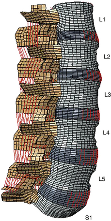
Even though the finite element method has been applied to structural engineering problems since the 1950s, it was first applied to the biomechanics of the spine in the 1970s.1,2 With improvements in numerical techniques and computer technology, its use in the field has gained momentum and it has become an integral part of spine biomechanics that is viewed as a complementary and insightful analysis (Fig. 22-1).
Modeling of Spinal Elements
Three-Dimensional Reconstruction and Structural Modeling
Several methods have been commonly used to model spinal units, including touch probe digitizer,3 laser scanner,4 CT,5 and MRI.6 Even though precise, highly accurate geometric models can be obtained using the touch probe digitizer and laser scanner methods, noninvasive techniques such as CT and MRI often are preferred because of their ability to retrieve data on internal features of the specimens—and even from live subjects—with ease. Some techniques also combine some of the methods mentioned earlier for the reconstruction of spinal units.7
In thorough finite element models, vertebral bodies usually are modeled in several sections, as cortical shell, cancellous core, dorsal bony elements, bony end plates, and cartilage layers, due to their unique material properties.5,7,8
In almost all studies, intervertebral discs are formed by three significant parts: the nucleus pulposus, the anulus fibrosus, and the cartilaginous end plates. The anulus is further divided into subcomponents such as ground substance and anulus fibers. Anulus ground substance is modeled as several layers surrounding the nucleus. The anulus fibers are angled 30 degrees and 150 degrees with respect to the transverse plane in adjacent layers.9,10 Some studies have used more realistic approaches in the design of these fibers by considering the increase in fiber angle from ventral to dorsal, and also fiber angle variation between anulus layers5,11 motivated by the histologic findings.12,13
After a solid model of the spine is built, each of its components is carefully divided into simpler substructures called “elements” for mathematical calculation purposes. Generally, hard tissues such as cortical shell, trabecular core, and dorsal elements are composed of tetrahedral (pyramid) and pentahedron (wedge) elements.14,15 With soft tissues, such as the anulus ground substance or cartilage layers, it is necessary to use hexahedral (rectangular prism) elements due to low-elasticity modulus and high Poisson ratio properties. In most studies, bilinear link or spring elements (cables), which are only capable of sustaining tension, are employed for ligaments and anulus fibers.5, 9–11
Material Definition
Vertebral Bodies, End Plates, and Facet Cartilages
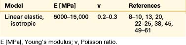
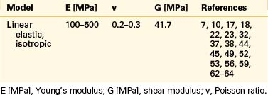
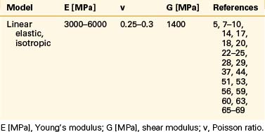
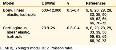
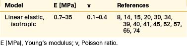
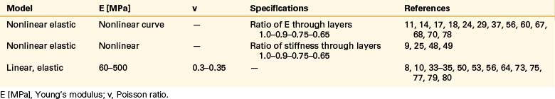
Even though bone is a poroelastic, anisotropic, and viscoelastic structure, in reality,16 vertebral cortical shell and cancellous bone usually are considered as linear elastic isotropic or transversely isotropic. Dorsal bony elements most commonly are modeled as linear elastic and isotropic (Tables 22-1 to 22-3). Researchers have either neglected the end plate due to its low elasticity module or modeled it as a composite structure (i.e., bony and cartilaginous layers). End plates most commonly were modeled as linear elastic and isotropic bone with a cartilaginous layer (Table 22-4). Cartilage layers also are added to the facets in most modeling paradigms (Table 22-5).
Intervertebral Disc: Anulus Fibrosus and Nucleus Pulposus
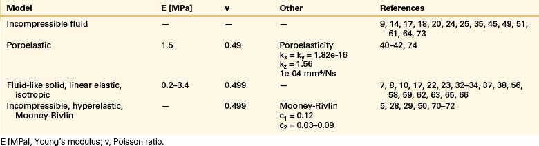
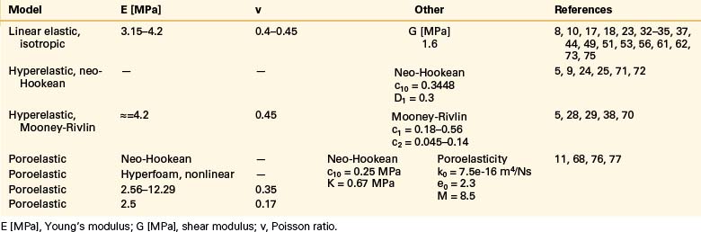
The intervertebral disc plays a crucial role in the movement and load-bearing functions of the spinal segments. It probably is the most intricate part of the functional spinal unit (i.e., vertebra-disc-vertebra complex) in finite element modeling, due to the composite structure of the anulus fibrosus and fluid-like behavior of the nucleus pulposus. The anulus fibrosus is formed by a matrix, anulus ground substance, and direction-dependent fibers. Even though there are a few homogeneous models for the anulus fibrosus, more realistic composite models that include matrix and angled fibers have been widely accepted and used (Tables 22-6 to 22-8). Anulus fibers are most commonly modeled with bilinear link, truss, or spring elements, and, in a few cases, with reinforced membrane elements. The material modeling of fibers is almost independent of the modeling technique.
Ligaments
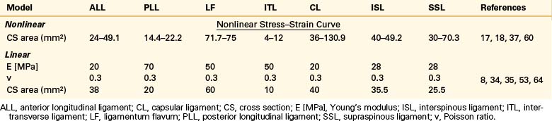
Ligaments are uniaxial structures that do not bear compressive loads. Like the anulus fibers, ligaments are modeled with link, truss, spring, or membrane elements. In general, it is assumed that linear, multilinear, or nonlinear elastic constitutive laws apply for these tissues (Table 22-9).
Articular Facet Joints
The facet joint plays an important role in load bearing and restriction of motion in segmental movements. It functions in tandem with the intervertebral disc in load transfer between adjacent vertebral bodies.17,18 The articulating structure must be modeled with realistic attributes and proper procedures in computational modeling of spinal segments because it has a significant effect on the quality and quantity of the motion. The articulation characteristics and relative motion depend on many factors, including cartilage layers, gap distance, the condition of the intervertebral disc, loading type, and geometric features of the articulating surface.
Kumaresan et al.19 compared different techniques for modeling of cervical facet joints. They reconstructed the joint capsule using four different methods: slide-line, contact plane, hyperelastic, and fluid models. The slide-line and contact plane models lacked the synovial fluid and synovial membrane. In the slide-line model, interaction was defined by using slide-line elements (gap elements), whereas in the contact plane model it was achieved by defining a contact plane between the cartilage surfaces. A friction coefficient of 0.01 was assigned for both models. The other models, hyperelastic and fluid, did not have elements for contact modeling; instead, they included synovial fluid between the cartilage layers modeled using noncompressible hyperelastic solid elements and hydrostatic noncompressible fluid elements, respectively. They concluded that fluid modeling of the facet joint matched both actual facet joint anatomy and its function better than the other three models. Similarly, Wheeldon et al.20 used full anatomic parts, such as facet joint cartilage, facet joint synovial fluid, and facet joint membrane, for modeling of the articular facet joints.
Shirazi-Adl et al.17,18 viewed the articulation process as a general moving contact problem and assigned 1 mm for the initial gap between the articulating surfaces. Guan et al.7,21 used 3D surface-to-surface contact to simulate the articulation phenomenon and assigned the initial gap between the surfaces according to CT images. Three-dimensional eight-noded compression-only gap elements were used to simulate the articulation between the facets in a study by Goel et al.22 Based on the CT images, they assigned the value of 0.45 mm for the initial gap between the surfaces.
The facet joints also are modeled with 3D gap contact elements with cartilage layers modeled using a parameter of “softened contact,” which exponentially adjusts force transfer between facet surfaces, according to the size of the gap.9,23–27 An initial gap of 0.5 mm was assigned, and at full closure, the joint was assumed to have the same stiffness as the surrounding bone material.
Schmidt et al.28,29 modeled the facet joints as nonlinear, with frictionless contact. They assigned the value of 0.6 mm for the initial gap between the cartilage layers. In other studies,30,31 the facet joints were simulated using frictionless surface-to-surface contact elements in combination with the penalty algorithm with a normal contact stiffness of 200 N/mm, and the initial gap between the cartilage layers assumed to be 0.4 mm.
Some researchers viewed the facet joints as a 3D contact problem with friction.8,32–34 To allow random motion of the surfaces, such as separation, sliding, and rotation, they defined a finite sliding interaction. For the friction characteristic, they chose a classic isotropic Coulomb friction model and assigned a relatively high friction coefficient of 0.1 as a worst-case scenario.
Lu et al.35 modeled the facet joints using sliding contact elements and assumed the contact pressure to be between 0 and 5000 megapascals (MPa), depending on the gap size. Pressure has been considered to be 0 MPa at a gap size of 0.5 mm and 5000 MPa when the gap is closed completely.
Loads and Boundary Conditions
Shirazi-adl et al.17,18 and Polikeit et al.8,34 applied a linearly varying distribution of axial loads to the top of the upper vertebra to simulate pure bending moments, with no net axial force. Kumaresan et al.36 and Wheeldon et al.20 succeeded in producing pure moments by using a force couple acting on the rigid plate attached to the superior vertebra.
Sharma et al.37 simulated pure flexion-extension moments using a pair of concentrated axial loads on top of the upper vertebra. They also studied the effect of anteroposterior shear during sagittal motion by a horizontal force applied at the center of the upper vertebral body. Two equal and opposite forces at the nodes at the edge of the sagittal or medial periphery of the upper vertebral body were applied to produce a force couple yielding a pure moment.38–42
Researchers have used the follower load technique, suggested by Patwardhan et al.,43 extensively for the last decade to simulate upper-body weight and the stabilizing effects of muscle forces seen in vivo without inducing any intervertebral rotations.9,25–28,30,44,45
Biomechanical Applications
Disc Degeneration and Vertebral Osteoporosis Simulation
In one of the earliest studies, Shirazi-Adl et al.45 modeled the degenerated disc by simply omitting a nucleus section. In another study, Shirazi-Adl et al.18 modeled the healthy disc as noncompressible fluid and suggested the loss of noncompressibility as a means to simulate the degenerated disc.
Goel et al.10 modeled the aging disc with a great deal of complexity by realistically simulating the radial and circumferential fissures in the anulus fibrosus that appear with age and discectomy. They simulated the radial crack in two ways: “out-in” injury started from the outermost layer and went through the innermost anulus layer with step-wise removal of the anulus elements, whereas “in-out” injury started from the innermost layer and went through the last layer of anulus simulated by replacing material of the anulus’s elements with nucleus material. They simulated the circumferential injury by removing the fourth anulus layer along the circumference, starting from posterior and extending through lateral.
Rohlmann et al.24 investigated the mechanical effects of three different grades of intervertebral disc degeneration—mild, moderate, and severe—compared with the healthy disc. They modeled the degeneration by reducing the disc height to 20%, 40%, and 60% of the healthy disc for mildly, moderately, and severely degenerated discs, respectively. In the finite element model, the laxity in all disc fibers and surrounding ligaments, seen on in vivo conditions after reduction of the disc height, was simulated by offsetting their nonlinear stiffness curves. They assigned the compressibility values for the nucleus pulposus of 0.0005, 0.0503, 0.0995, and 0.15, respectively, for healthy disc and mildly, moderately, and severely degenerated intervertebral discs. They assumed no effect on the material properties of the anulus fibrosus from degeneration of the disc.
Hussain et al.41,42 modeled two different degenerated discs, moderately and severely degenerated, to study the effects of disc degeneration on the facet loads. They simulated the degeneration according to the signs of Thompson disc grades 2 and 3 (moderate) and 4 and 5 (severe). They decreased the disc height, increased the disc area, and reduced the nucleus portion to simulate the degenerated disc. They also reduced the Poisson’s ratio in severely degenerated discs and increased the Young’s modulus of anulus and nucleus in both moderately and severely degenerated discs.
Galbusera et al.11 meticulously modeled the degeneration of the disc based on five different degenerative characteristics: (1) loss of water content in nucleus and anulus, (2) calcification and thickness reduction in end plates, (3) loss of disc height, (4) formation of osteophytes, and (5) diffuse sclerosis. They obtained ten different spinal segments by scaling the size of the finite element model to represent different stages of each degeneration level (mild, moderate, and severe). They changed the initial void ratio to model the degeneration in the nucleus and anulus, and they formed three different types of anular lesions: a rim lesion, a radial tear, and a circumferential tear. They modeled end plate cartilage degeneration by reducing its height and changing its material properties. Degeneration of the disc also was modeled with reduction of its height. When simulating the osteophytes, they used solid elements with the same material attributes of bone and anulus between them. They simulated sclerosis by interchanging the material properties of cancellous bone with the cortical bone in certain areas. They divided the lower half of L4 and the upper half of L5 into four regions and randomly assigned the sclerosis deficiency to these sections.
Polikeit et al.46 investigated the effects of osteoporosis and disc generation on the load transfer characteristics of an L2-3 segment. Initially, they modeled an osteoporotic vertebra by decreasing the elasticity modulus of trabecular bone by 66% and other bony parts by 33% compared with healthy model. Next, they simulated the progress of osteoporosis by modeling the cancellous bone transversely isotropic (i.e., the elastic modulus in the horizontal direction was one third of that in the vertical direction, using the same material properties as for the isotropic case) and increasing the anisotropy gradually. They postulated five steps of degeneration based on the isotropic osteoporotic vertebra model. At the first step, they changed the material definition of the nucleus pulposus from noncompressible to deformable. In the second step, the nucleus pulposus was hardened by assigning the same material properties as the ground substance of the anulus, and subsequently the Young modulus of the whole disc was doubled. In the fourth step, the innermost anulus layer was removed, other layers were thickened, and increased space between the fibers resulted. In the last step, they further reduced the elasticity modulus of the last remaining fiber layers. They also modeled a worst-case scenario by using transversely isotropic osteoporotic vertebral bodies in conjunction with the degenerated intervertebral disc.


Stay updated, free articles. Join our Telegram channel

Full access? Get Clinical Tree


