Chapter 4 Electroencephalographic Localization

It is easy to underestimate the importance of learning the skills of precise EEG localization compared with the bigger picture of EEG interpretation. On the face of it, the purpose of localization is to identify the location in the brain at which a recorded EEG event has occurred. Indeed, if this were the only benefit of learning accurate localization, it would still be a key skill in EEG interpretation. However, as we shall see in this chapter and elsewhere in this text, localization can help answer not only where an EEG event has occurred but also what an EEG event is. Understanding the topography and polarity of a discharge is the first step in deciding whether an EEG event is truly of cerebral origin or is instead an electrical artifact. Consider for a moment the potential negative impact on patient care of reporting an electrical artifact as an abnormal cerebral discharge. As we shall see, the shape or distribution of certain EEG discharges may not be consistent with cerebral activity because the localization does not make either topographical or biological sense. The skill of accurate EEG localization includes the skill of determine whether the shape or distribution of a discharge is or is not consistent with an event that originates from the brain. In addition, certain discharge topographies can suggest a specific type of discharge and the clinical syndrome to which the discharge might belong; in certain cases, the location of the discharge can reveal what it is.

Complete localization of an event includes pinning down both the event’s location and its polarity. For instance, an accurate localization would include not only the fact that an event occurs in the left anterior temporal electrode but also whether it is negative or positive at the scalp surface. Almost all types of EEG events can be localized, whether they be spikes, sharp waves, slow waves, or even voltage asymmetries. In the following discussion, the examples used are spike-like discharges, although the principles discussed here apply equally well to almost all types of EEG events (e.g., sharp waves, slow waves, etc.).

FOCAL EVENTS, ELECTRIC FIELDS, AND GENERALIZED EVENTS

Focal Events

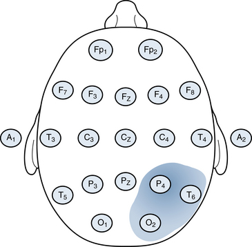
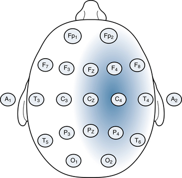
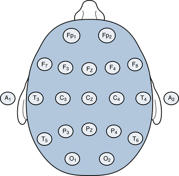
A focal EEG event is one that occurs on a limited part of the brain surface rather than over the whole brain surface. Occasionally, an event may be so focal that it occurs in only one electrode. The large majority of discharges will also be detectable, though perhaps more weakly, in adjacent electrodes. The electrode position that picks up the highest voltage, be it positive or negative, is referred to as the discharge’s maximum. Although the discharge may be best seen at the maximum, adjacent electrodes often pick up varying amounts of the discharge. The hypothetical discharge shown in Figure 4-1 shows a discharge maximum in the right parietal electrode (P4) with a field that includes the right posterior temporal electrode (T6) and, to a lesser extent, the right occipital electrode (O2). A focal discharge having a broader field, such as the one shown in Figure 4-2, can have a maximum at one electrode (C4 in this example) but involve a substantial part of one hemisphere.

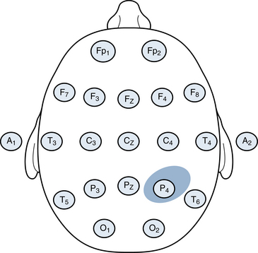
Figure 4-1 This focal discharge is clearly maximum in P4, but the electric field of the discharge extends to include T4 and O2. Rather than seeing a discharge occur at a single electrode position, this is the more common situation in which the maximum of a focal discharge is picked up in one location (P4 in this example) but the discharge can be detected to a lesser extent in adjacent electrodes (T6 and O2). In this case, the discharge can be said to be maximum in P4 with a field that extends to T6 and O2.

Figure 4-2 In the case of a lateralized discharge, the field of the discharge involves either a whole or nearly whole hemisphere. In this example, the discharge can be said to be lateralized to the right hemisphere.

Rarely, an EEG event may occur so focally that its activity is only recorded in a single electrode, such as the example of the highly focal right parietal discharge shown in Figure 4-3. According to the schematic, the discharge would only be detected by the single electrode (P4), and adjacent electrodes would be electrically quiet. In practice, such highly focal discharges are uncommon and represent the exception rather than the rule (although this phenomenon of highly focal discharges is more commonly seen in newborns). The first two examples given above in which a discharge is detected by a group of electrodes is the more commonly encountered situation. The pattern of how strongly the discharge is picked up in various electrodes helps define the shape of the discharge’s electric field as discussed next.

Figure 4-3 The discharge depicted here is highly focal and is only detected by a single electrode (P4). The adjacent electrodes are electrically “quiet.” This highly focal pattern is relatively uncommon; most focal discharges affect multiple electrodes at once. When an event is limited to a single electrode, the possibility of an electrode artifact should be considered.

Electric Fields

Several analogies have been used to describe the shape of the electric field of a typical discharge on the scalp surface and how its intensity drops off with distance from the maximum. The analogy of a pebble dropped into a quiet pool of water can be used to describe the way a simple field’s strength dissipates as it becomes more distant from the point of highest intensity (where the pebble hit the water). The wave that is formed is strongest at the point of impact but diminishes with increasing distance from the central maximum. This example is useful because many electric fields measured on the scalp do show this radially symmetric shape but, in practice, many electric fields dissipate with varying shapes.

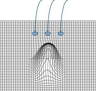
Rather than showing a smooth and steady decrease in voltage in every direction from the central maximum point, it is possible for fields to dissipate gently in one direction and abruptly in another. A better analogy for the shape of electric fields is the visualization of mountain peaks. Mountain peaks give a more realistic picture of EEG fields because they need not be so perfectly symmetrical in shape as the circular waves caused by a pebble hitting water. Imagining the terrain around a 5,000-foot mountain peak, we might expect that the height of land surrounding the peak will fall off with varying steepness in each direction. Likewise, electric fields may manifest a steeper slope of voltage decrease in one direction and a more gentle slope in another direction. An abrupt and immediate falloff in voltage from a central point in all directions as shown in Figure 4-4 would correspond to a thin needle of land 5,000 feet high with nothing surrounding it, an uncommon finding both in geography and in electroencephalography but akin to the discharge in Figure 4-3.

Figure 4-4 This schematic illustrates three electrodes recording over a highly focal discharge. Note that because of the pinpoint location of the discharge, only the middle electrode detects a change in voltage.

The mountain peak analogy reminds us that an electric field can be visualized as a surface in three dimensions. Just as slope refers to the steepness of a curve imagined in two dimensions at a given point, the steepness of a surface imagined in three dimensions at a given point is referred to as the gradient at that point. (The slope of a curve at a given point is the slope of a line tangent to that curve at a given point. Similarly, the gradient of a surface at a given point is defined by the slope of an imaginary plane tangent to the surface at that given point.) The rate at which the terrain that surrounds the summit of a mountain falls off is the steepness of the terrain. The rate at which an electric field changes intensity at a particular point on a surface is called the electrical gradient; the two properties are analogous. The exercise of visualizing the shapes of electric fields is similar to visualizing the contours and steepness of a region of mountain terrain. Just as we would never confuse the area of maximum altitude of a mountain with the point of maximum steepness of a mountain (which may or may not be at the same point), so we will take care not to confuse the point of maximum voltage of an EEG event with the point of the maximum gradient of the field surrounding the maximum.

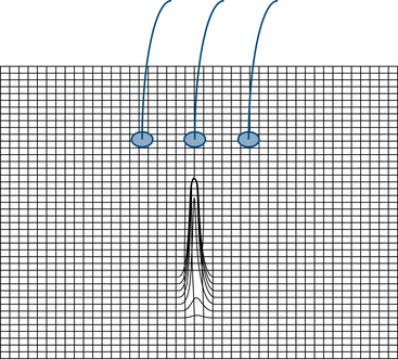
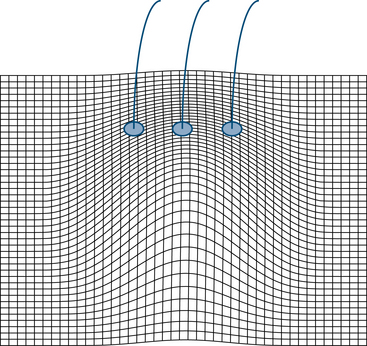
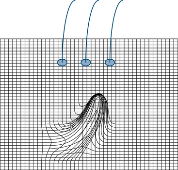
The illustration in Figure 4-4 depicts a highly focal discharge, similar to that shown in Figure 4-3. The plane of the rectangular grid is a representation of the voltages measured on the scalp surface. In this figure, areas close to the discharge’s peak are not involved, and relatively nearby electrodes would not “perceive” any change in voltage. Such highly restricted or “punched-out” discharges are relatively uncommon (just as 5,000-foot mountains in the shape of a needle are uncommon). The field shown in Figure 4-5 is somewhat more realistic, with a peak or maximum in the same position, but a more gradual falloff in voltage as distance increases from the maximum point. In this example, adjacent electrodes would pick up increasingly weaker voltages with increasing distance from the point of maximum. Figure 4-6 shows a discharge with a broad field, and, although the middle electrode would pick up the highest voltage, the adjacent electrodes would detect a voltage intensity of more than half that detected by the middle electrode. Figure 4-7 reminds us that, quite often, the electric field can slope off asymmetrically from its peak.

Figure 4-5 The discharge depicted here has a more broadly sloping electric field, and although the middle electrode picks up the biggest voltage change, adjacent electrodes pick up lower voltage changes on the “shoulders” of the field.

Figure 4-6 Again, the middle electrode picks up the maximum voltage change, but the adjacent electrodes also pick up a significant portion of the discharge on the slopes of its electric field.

Figure 4-7 The intensity of the field of this focal discharge slopes off more steeply in some directions and more gradually in others. Such asymmetric gradients are common.

Generalized Events

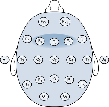
In contrast to the focal events described earlier, some events occur in all brain areas at once and are said to occur in a generalized distribution. Figure 4-8 depicts a discharge with a perfectly even electric field. With cerebral discharges, even in the case of generalized discharges, there is almost always some unevenness to the field, and an area of maximum intensity can still be identified. In Figure 4-9, the discharge affects all brain areas and is, therefore, generalized, but the intensity is highest in the F3, Fz, and F4 electrodes.

Figure 4-8 This is a depiction of an idealized generalized discharge. The shading of this figure implies that the event is distributed in a perfectly even fashion, although in actual recordings, some amount of unevenness is usually seen even in the fields of generalized discharges.

Figure 4-9 This generalized discharge has a clear maximum in the superior frontal and midline frontal electrodes, F3, F4, and Fz. This is a common localization pattern for the “classic generalized spike-wave” discharge.

The purpose of this chapter is to help the reader become adept at translating the patterns of pen deflections recorded on the EEG page into the particular localizations, polarities, and the shapes of the gradients that those patterns imply. In short, we examine the patterns that EEG pens will draw when they encounter electrical fields of various shapes, including the types depicted in the figures discussed earlier. Ideally, after analyzing an EEG discharge on an EEG page, the reader will be able to imagine a “mountain range” configuration that accurately depicts the shape and the gradients of the discharge’s electric field.

EEG WAVES AND EEG POLARITY

Pen Up or Pen Down?

An understanding of what causes the EEG instrument’s pen to go up or down is the foundation concept of EEG localization and is one of the central skills to master in this chapter. Luckily, the convention is easy to understand. The challenge is to remember to apply it consistently when analyzing EEG patterns.

EEG Channels Are Fancy Voltmeters

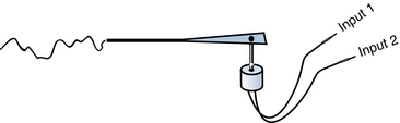
A voltmeter measures the potential difference or “voltage drop” between two points. Because voltages are always differences, whenever a voltage measurement is made, the reader should be aware which two identifiable points are being compared. Even when it appears that the voltage at a single point is being described, it is implicit that the point is being compared with some standard (perhaps a ground or other “neutral” point). Likewise, even though there may be a temptation to think of the output of an EEG channel as representing the activity at some single point on the scalp, every channel deflection we see on the EEG is, in reality, a comparison of two different points on the body (or occasionally a combination of more than two points, as we shall see in later chapters). Any wave seen on the EEG is, therefore, a comparison of the electrical potential at two locations rather than an absolute measurement made at a single location. The waves that we are analyzing are, indeed, the outputs of constantly fluctuating voltmeters comparing two inputs (see Figure 4-10).

Figure 4-10 An EEG channel can be thought of as the pen output of a continuously recording voltmeter with the two inputs specified by the recording montage in use.

Inherent to the concept of the voltmeter is the idea of subtraction. If one probe of a voltmeter contacts a point at 105 μV and the second probe contacts a point that is at 100 μV, the voltmeter will read out 5 μV. Likewise, if the pair of points recorded is −112 and −117 or even 3 and −2, the voltmeter will read out the same result: the difference of 5 μV. The result of 5 μV that the voltmeter yields gives no clue as to which of these pairings generated it: 105 and 100, −112 and −117, or 3 and −2. The fact that an EEG channel only shows us the difference between two points rather than absolute values has both advantages and limitations. Because each wave displayed on the EEG is a continuous voltmeter output, the reader should always have in mind the following question: which two points are contributing to this channel’s appearance?

The reader may be wondering which would be more logical, for the pen to go up or for the pen to go down, in the example in the preceding paragraph in which the difference is positive 5 μV. The answer to this question cannot be derived using mathematical or physical principles. Rather, it is an arbitrary convention that was decided by EEG machine manufacturers in the early days of EEG. The answer for the earlier example is that the pen goes down. The convention assumes that there are two input terminals to the amplifier, Grid 1 and Grid 2, which can also be called Input 1 and Input 2. The convention is: “First input more negative: pen goes up. First input more positive: pen goes down.” Some may find this convention counterintuitive because in most areas of mathematics and science, values are graphed above the x axis when they are positive and below the x axis when they are negative. Alas, in electroencephalography, the opposite is true; this “upside-down” convention is here to stay and can take some getting used to. It may be helpful to use the counterintuitive nature of the convention to help remember it.

Here is how the convention works in more detail: as noted, every EEG amplifier has two principle inputs, which we will refer to as INPUT 1 and INPUT 2. The EEG technologist decides which electrodes are plugged into INPUT 1 and INPUT2 for any given channel according to which EEG montage is chosen. The situation of INPUT 1 being more negative than INPUT 2 can be stated in a number of ways, such as: “the difference between INPUT 1 and INPUT 2 is negative” or as the mathematical expression: “INPUT 1 − INPUT 2 < 0.” In such cases the amplifier’s pen deflects upward. Of course, the opposite holds true for the reverse situation: when INPUT 1 is more positive than INPUT 2, the pen deflects downward as in the example above (see Figure 4-11).

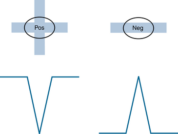
Figure 4-11 The convention for pen movement is best memorized on the basis of the INPUT 1 electrode or “Electrode 1.” When Electrode 1 is more positive than Electrode 2, the pen goes down. When Electrode 1 is more negative than Electrode 2, the pen goes up. For this reason, in referential montages in which the electrode of interest is attached to INPUT 1 and a “neutral” reference electrode is attached to INPUT 2, negative events on the scalp appear as upgoing deflections.

When INPUT 1 is more positive than INPUT 2, the pen goes down.

When INPUT 1 is more negative than INPUT 2, the pen goes up.

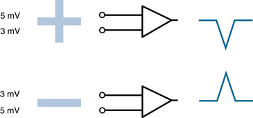
Of all the ways to state this rule, the subtraction expression “if INPUT 1 − INPUT 2 > 0 . . .” is most correct because it deals with all the possible combinations of each of the two inputs being positive, negative, or zero. One could quibble with the idea of saying that −3 is “more positive” than −5 because neither is positive. In this text, we use this simpler shorthand, stating that one electrode is “more positive” or “more negative” than another without regard to the sign of the electrodes’ absolute voltages for simplicity’s sake. Figure 4-12 shows another representation of this convention.

Figure 4-12 When the common mode rejection amplifiers used in EEG recording encounter a “more positive” voltage in INPUT 1 compared with INPUT 2, the pen goes down as is seen in the top example. Likewise, when the voltage in INPUT 1 is “more negative” compared with INPUT 2, the pen goes up, as is seen in the bottom example. The top example shows a 5 μV wave presented to INPUT 1 and a 3 μV wave presented to INPUT 2. The difference is positive, and, by convention, the pen goes down. The bottom example shows the result of switching the input voltages. Now the difference between INPUT 1 and INPUT 2 is negative, and the pen goes up.

EEG Amplifiers

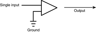
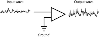
To understand the meaning of pen deflections, it is useful to consider the nature of the amplifiers used in the electroencephalograph. Perhaps the simplest conceivable amplifier design would be the single-end input amplifier. This type of amplifier would take a single signal as its input and furnish an amplified version of that signal as its output (see Figures 4-13 and 4-14). This is not, however, the type of amplifier used in EEG machines, and for good reason. A single-end amplifier is essentially using the building’s electrical ground as the comparison input; however, such grounds are usually much too electrically contaminated or “dirty” to be useful for this purpose.

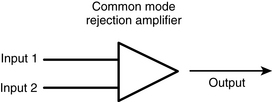
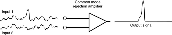
Figure 4-13 A single-end amplifier takes a single active input and compares it to electrical ground, theoretically an electrically neutral position, and amplifies the difference. In practice, building grounds are often contaminated with significant amounts of electrical noise from other devices attached to the ground at other locations. When compared with and subtracted from the weak EEG signals in the single active input, the noisiness of the ground could swamp the low-voltage brain wave signal.

Figure 4-14 This idealized single-end amplifier takes a single signal as input and outputs an amplified version of the same signal. This is not the type of amplifier setup used in EEG machines.

Actual EEG amplifiers, like the voltmeters described earlier, use two inputs (see Figure 4-15). The signal from INPUT 2 is subtracted from the INPUT 1 signal; the result is then amplified and serves as the output. This type of amplifier is also called a common mode rejection (CMR) amplifier. As we shall see, the strategy of subtracting one input signal from the other has several important advantages. Figure 4-16 shows how a CMR amplifier behaves with two sample electrical inputs. Note that the component of each signal that is common to both inputs is cancelled out, or “rejected.” Only the difference between the two signals appears in the output. Why is elimination of the part of the signal that is common to both electrodes an advantage? This technique of amplification is especially useful in the field of electroencephalography in which the signals of interest—brain waves—are of very low voltage compared with the ambient electrical noise from external sources that runs through the patient’s body. Because the pattern of this external noise signal tends to be similar in the various scalp electrodes, CMR amplifiers cancel out much or all of the external noise component of the signal, ideally leaving only the cerebral component for interpretation.

Figure 4-15 The common mode rejection amplifier accepts two inputs, each usually from a single electrode, and yields a single amplified output.

Figure 4-16 An idealized view of a CMR amplifier processing two signals. Note that there is a single difference between the INPUT 1 and INPUT 2 signals, a single upward deflection. The complex underlying waveform is common to both inputs and, when the two signals are subtracted, is cancelled out or “rejected.” The “difference signal,” consisting of the upward deflection, is amplified and represents the output. In this example, one can imagine that the waveform recorded from INPUT 2 is obtained from a location such as the earlobe and consists solely of electrical noise. The signal recorded from INPUT 1, which has been placed on the nearby scalp, is contaminated by the same electrical noise as the earlobe but also contains a single “brain wave,” the upward deflection. The result of the CMR amplifier’s action is to subtract out the noise signal and display an amplified brainwave.

Event Localization Using a Bipolar Montage

The examples that follow consider a theoretical spike discharge on the scalp and how it would appear on the EEG record. The first example we examine is a hypothetical spike in the left central region of the brain (the area under the C3 electrode). A spike is, by definition, a quick event, and in this example, it will have a negative polarity (the scalp region where the spike occurs will be momentarily negative compared with the surrounding scalp, which, for the purposes of this example, is neutral). The electrode set we use to record the spike is a single chain of standard electrodes that goes along the scalp from front to back just to the left of the midline: Fp1, F3, C3, P3, and O1 (the left frontopolar, superior frontal, central, parietal, and occipital electrodes, respectively). The technique used for the following examples is the typical strategy of creating a bipolar chain with these electrodes by looking at a succession of pairings of adjacent electrodes from front to back: Fp1 to F3, F3 to C3, C3 to P3, and P3 to O1. The term bipolar is used because each EEG channel generated represents a comparison of two cerebral locations. Each of the two electrode locations can be said to be “of interest” because both reflect brain activity, and it is possible that a clinically important event could arise from under any of the five electrodes. (In the contrasting situation of referential montages described in more detail later, INPUT 1 is connected to an electrode over the brain, and INPUT 2 is connected to some other reference point that is presumably not “of interest” but is used for the purpose of subtracting noise.) Note that there are five electrodes in this chain but there are necessarily only four consecutive pairings. Thus, a chain of five consecutive electrodes will produce four channels of EEG in a bipolar chain.

“Negative Phase Reversal”

Figure 4-17 depicts the field of a 50-μV spike occurring at C3 with no activity at all in the surrounding electrodes. On the right, the four channels representing the output of the bipolar chain are depicted. It is worthwhile to go through each line of the output to understand exactly why voltage measurement shown on the left side of the figure is associated with the EEG trace on the right side of the figure.

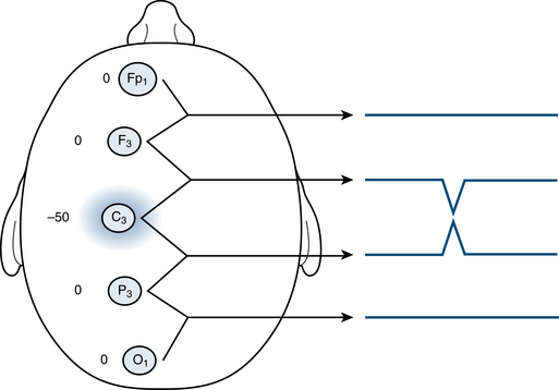
Figure 4-17 A negative phase reversal showing a focal negatively charged spike occurring only in the C3 electrode—none of the negativity of the spike is picked up in adjacent electrodes. The numerical voltages that each electrode detects are shown. The dark shading denotes the region of the scalp that becomes negatively charged during the spike. The resultant EEG trace seen in a bipolar chain (Fp1-F3, F3-C3, C3-P3, and P3-O1) is shown to the right and the reasons for each specific pen deflection are described in the text.

The first channel, Fp1-F3 is measuring the difference between 0 μV at Fp1 and 0 μV at F3. Because there is no difference, the Fp1-F3 channel remains flat.

The second channel, F3-C3, is comparing 0 μV in INPUT 1 (F3) and −50 μV in INPUT 2 (C3). Because the convention is that if the first electrode is “more positive” than the second, the pen goes down, a downward pen deflection is produced.

The third channel, C3-P3, compares −50 μV in INPUT 1 to 0 μV in INPUT 2. Now Electrode 1 is more negative than Electrode 2 (the opposite of what occurred in the second channel), so the convention tells us that the pen goes up.

Finally, in the fourth channel, there is no voltage difference measured between P3 and O1 (both 0 μV), so the channel remains flat.

The resulting trace shows one of the classic patterns of EEG waves, the phase reversal, which is expanded on below. For the time being, note that, in this example, where the pen deflection reversed direction, or phase (in this case from down in the second channel to up in the third channel), the electrode in common to the channels where the phase reversed from down to up (C3 since the phase reversed between F3-C3 and C3-P3), points to the location of the discharge’s maximum.

As discussed earlier, focal EEG events on the brain surface rarely occur solely in an isolated pinpoint area of the scalp as in the example in Figure 4-17. Instead, there is typically a point of voltage maximum around which lower voltages can be detected. The example shown in Figure 4-18 is more similar to real-world events. Although the C3 electrode is the point of maximum intensity of this event, the adjacent areas measured by F3 and P3 are also affected, but not as strongly. This gradual drop-off in intensity of voltage shows that the event has a somewhat broader field, even though we are still dealing with a −50-μV spike in C3. A good description of this spike would be that the spike has a maximum negativity at C3 but a field that also includes F3 and P3.

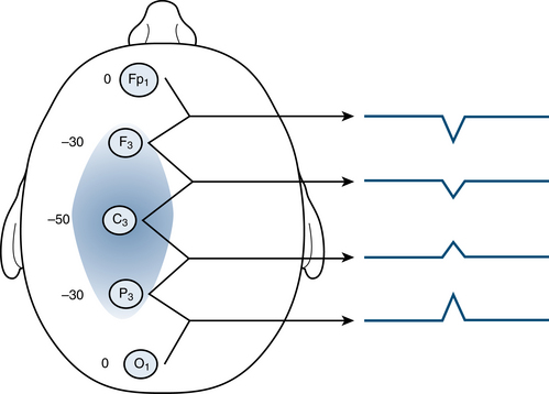
Figure 4-18 A –50-μV spike in C3 with a field extending to include F3 and P3 viewed in a bipolar montage. The F3-C3 and C3-P3 channel deflections reflect the 20-μV difference between those electrode pairs. The higher deflections seen in the top and bottom channels, Fp1-F3 and P3-O1, reflect the 30-μV gradient between those electrode pairs.

Now let’s return to Figure 4-18, which shows a more realistic gradient around a spike focus at C3. The resulting EEG trace is similar to the one we saw earlier but with some notable differences:

The first channel, Fp1-F3, is measuring the difference between 0 and −30 μV. Because Electrode 1 is “more positive” than Electrode 2, the pen deflects downward an amount corresponding to the difference of 30 μV.

The second channel, F3-C3, compares −30 μV in Electrode 1 (F3) and −50 μV in Electrode 2 (C3). Because the first electrode is again “more positive” than the second, a downward pen deflection is produced in this channel as well, corresponding to the smaller difference of 20 μV.

The third channel, C3-P3, compares −50 μV in Electrode 1 to −30 μV in Electrode 2. For the first time, Electrode 1 is more negative than Electrode 2 (the opposite of the case in the second channel), so the convention tells us that the pen now goes up.

Finally, in the fourth channel, Electrode 1 measures −30 μV, and Electrode 2 measures 0 μV. The pen again deflects upward, corresponding to the fact that Electrode 1 is more negative than Electrode 2 by a 30-μV difference.

Comparing the pattern of EEG waves in Figure 4-18 to the previous figure, we see that there are now deflections in all four channels. This reflects the fact that the field of this spike involves both adjacent electrodes, F3 and P3, and that the gradient of the field stretches out more broadly than in the first example. Stated another way, there is now an electrical gradient (difference) between all four channel pairs. The fact that there is a deflection in each channel reflects the fact that no two adjacent electrodes measure the exact same voltage and that there was an increase or decrease in voltage in every comparison. Because in channels 1 and 2 the pen goes down and in channels 3 and 4 the pen goes up, we say there is a phase reversal occurring between channels 2 and 3. A phase reversal is the point along a bipolar electrode chain at which the direction of the pen deflection changes (from down to up or from up to down). Because in this example C3 is the electrode common to channels 2 and 3, the two channels between which the phase “reversed,” this is the point of maximum of the discharge.

A second interesting observation can be made about this recording. Even though the biggest pen deflections can be seen in channels 1 and 4, the true maximum of the discharge lies between channels 2 and 3. This apparently paradoxical result occurs because, in this example, the electrical gradient was steeper at some distance from the maximum (nearer the forehead and occiput), similar to the example of a mountain peak in which the terrain could be steeper around the base of the mountain and less steep as it reaches its peak. Still, the “peak” is at C3, even though the deflections in Fp1-F3 and P3-O1 are larger. Clearly, in bipolar montages the maximum of a discharge cannot be located simply by finding the biggest waves—a pitfall to be avoided. This is because the measuring stick used to determine wave heights in bipolar montage tracings is the differences between pairs of points rather than the absolute value of the voltage at any given point. In bipolar montages, rather than using wave heights, the maximum is located by finding the phase reversal.

Each EEG channel in a bipolar chain passing from front to back along the head is, in reality, answering the question in its march along the brain: “is the next electrode getting more negative or more positive?” The following analogy illustrates this effect another way: a farmer has a large field and would like to build his house at the highest point in the field to have the best view of his farm from his house. The farmer does not have a standard instrument to measure height (an altimeter), and he does not trust himself to find the highest point using standard visual inspection. Rather, the only tool he can use to locate the highest point in the field is a crude instrument that only reports the difference in height of his current position compared with his last position as he takes steps across the field. It can inform him that the field has gotten higher compared with his last location (in which case its pen goes down) or that the field has gotten lower compared with his last location (in which case its pen goes up). He takes readings every time he walks 10 feet forward. Even without having the benefit of an altimeter that could report absolute numerical altitudes, as he walks forward through his field, it is easy to imagine a strategy he can use to locate the highest point along any track he walks.

Imagine that the farmer turns on the instrument (which senses his starting position) and then walks forward the first 10 feet. The instrument, comparing the starting position to his present position, reports “it’s getting higher” (the pen goes down). After the next 10 feet, it reports that it is getting higher again (the pen goes down again). After the next 10 feet, it reports “it’s getting lower” (the pen now goes up). This is the point of the “phase reversal” when the pen direction has changed. The farmer does not know the absolute altitude at the previous point, but he does know that the area between the points at which his instrument”s pen flipped from down to up must mark the highest point on the track he has walked so far. After the pen readings shift from downward to upward, he knows he has located a height maximum along the line he is exploring. This is the equivalent of a phase reversal in a bipolar chain on the EEG. Before making a final decision, he will probably want to get to the end of the field to make sure that he found the highest point on the whole path. If he wanted to make a topographic map of the whole field, he could perform the same top to bottom walk along the field in several parallel lines. To be even more complete, he might repeat the measurements walking on parallel tracks from right to left (at right angles to the original paths). Using this strategy and recording the amount his pen deflects on every measurement, he would eventually be able to draw a relative topographic map of the whole field, something like the grid shown in Figure 4-6.

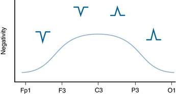
In these examples, greater altitude in the farmer’s field is analogous to EEG voltage becoming more negative. The EEG reader can imagine “walking down” or scanning a bipolar chain along the scalp such as from Fp1 all the way to O1 and, like the farmer, feel as the pens go down that “it’s getting more negative” and then as the pens finally reverse direction that “it’s getting more positive.” When the pens switch direction, this implies that the point of maximum negativity was passed, identifying the position of the maximum voltage of the spike. Figure 4-19 shows the deflections that the farmer’s instrument might generate while walking along a single path, or likewise what an EEG machine might detect when exploring the parasagittal chain when there is a spike maximum at C3.