Very Fast and Very Slow Activity

Although the list above implies that beta-range frequencies are unbounded on the high side, in reality EEG activity recorded at the scalp with routine EEG instruments rarely exceeds 30 to 40 Hz, and even signals from cortically implanted electrodes rarely exceed 50 Hz. High-frequency filtering techniques and other inherent equipment limitations make it difficult to see faster frequencies in routine recordings, even should they be there to record. The assumption behind using high filters is that little or no cerebral activity exceeds 30 to 40 Hz so that any signals above this range likely represent electrical noise or “artifact” from muscle, electrical interference, or other sources—hence, the strategy to filter out most activity above this range. In the early days of EEG, frequencies above 30 Hz were said to be in the gamma range, but the term (and the concept) was later discouraged. More recently, there has been renewed research interest in “gamma activity,” although such very fast activity has yet to establish its place in the mainstream of conventional EEG interpretation.

Similarly, although the lower bound of the delta frequency range is “zero Hz,” it was initially felt that there was little cerebral activity below 0.5 Hz. Newer techniques have successfully recorded very slow activity, which are termed DC potentials because they resemble shifts of the baseline (direct currents) rather than oscillations. Again, because standard recording techniques usually exclude most such very slow activity, frequencies much below 0.5 Hz are usually not reliably observed in conventional EEG recordings. Despite the possible existence of some very slow potentials in the EEG, in some situations, the great majority of activity below 0.5 Hz usually represents motion or electrical artifact rather than electrocerebral activity. Conventional filtering techniques attempt to remove these large baseline shifts from the recording because they usually represent artifact and may render the EEG tracing unreadable (see Chapter 7, Filters).

The term slow activity refers to any waves for which the frequency falls below the alpha range (i.e., delta and theta activity—activity below 8 Hz). Likewise, the term fast activity refers to activity for which the frequency lies above the alpha range (i.e., beta activity–activity above 13 Hz).

A Note on Units

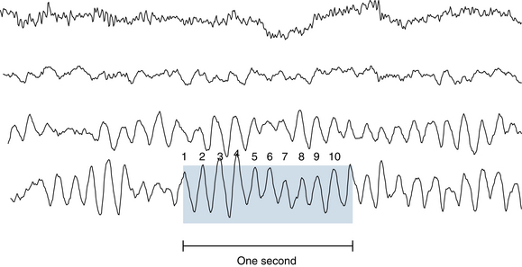
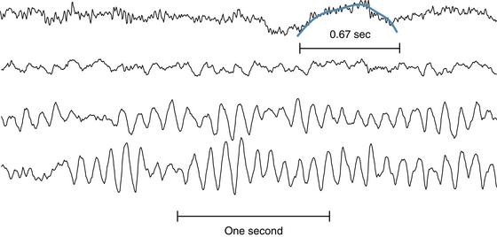
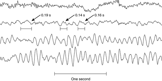
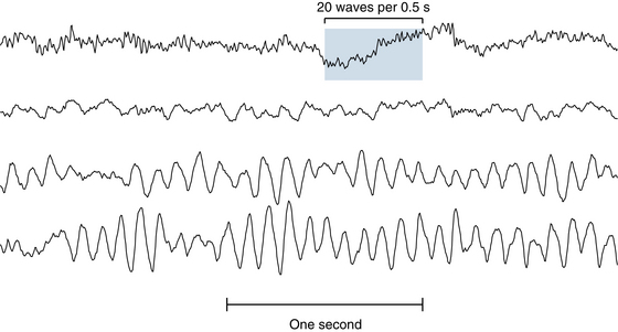
The foregoing examples assume that wavelengths are stated in seconds, but it is common practice to quote wave durations in milliseconds (msec). Rather than stating that a wave lasts 0.2 seconds, it is often said that the wavelength is 200 msec. Using milliseconds is perfectly satisfactory, except when it comes to using the formula cited earlier to calculate frequency. The reciprocal of 200 is 0.005, which clearly is not the correct frequency of a wave of 200 msec duration. This is because inserting a wavelength in milliseconds into the formula yields the result in the undesirable unit of “cycles per millisecond.” To yield the frequency in cycles per second, or Hertz, the wavelength used in the formula must always be stated in seconds (1 cycle/0.2 sec = 5 cps). Examples of how the frequency of alpha, delta, theta, and beta activity are assessed are shown in Figures 3-1 through 3-4.

Figure 3-1 The frequency of the wave in the blue rectangle is most easily determined by counting the number of wave peaks or troughs seen in 1 second. These waves are rhythmic, fairly sinusoidal in shape, and vary in amplitude. In this example, 10 wave peaks are counted in a 1-second time period, indicating that this is an example of fairly regular 10-Hz alpha activity. This particular tracing represents an example of the posterior rhythm of a 7-year-old boy.

Figure 3-2 The frequency of the nonrepeating slow wave denoted by the penstroke in the top channel is most accurately assessed by measuring its wavelength. The wave in this example is 0.67 seconds in duration, measured from wave trough to wave trough. The simple relationship of wavelength to frequency described in the text in which frequency is the reciprocal of wavelength (1 cycle / 0.67 seconds = 1.5 cycles per second) tells us that this is a single 1.5-Hz delta wave. Note that the wave’s frequency can be determined even though it stands alone and does not repeat, and also that the shape of this slow wave can be seen despite the superimposed fast activity. If a wave of this size did repeat, it can be visually estimated that 1.5 such waves would fit into 1 second.

Figure 3-3 The frequency of irregular theta waves can be assessed using the same technique of measuring wavelength that was used for the previous figure. In the second channel of this figure, several semirhythmic theta waves can be seen with the durations shown in the figure. Although the waves indicated by the arrows do suggest some rhythmicity, each varies to some extent in wavelength and cadence. By calculating their reciprocals, the measured wavelengths of 0.19, 0.14, and 0.16 seconds correspond to frequencies of 5.3, 7.1, and 6.3 Hz, respectively, all of which are in the theta range (4–8 Hz).

Figure 3-4 The fast activity seen in the shaded area of the first trace is too fast to make an accurate measurement of wavelength and would be cumbersome to count for a full second. Here, in the half-second interval denoted by the shaded rectangle, 20 waves are counted, implying a frequency of 40 Hz. Given the high frequency of these waves and the fact that they were recorded over the frontalis muscle, these may represent an example of electrical muscle artifact.

Waves of Mixed Frequency and the Fourier Theorem

The foregoing discussion deals with descriptions of simple waves of a single frequency. However, after a brief look at actual EEG recordings, it is clear that few, if any, of the waveforms seen on the EEG page resemble the pure sine waves seen in math textbooks. Indeed, as a rule, EEG waves represent a mixture of waves of different frequencies and amplitudes. Part of the reason for this mixture of frequencies is that the waveform recorded at the scalp often consists of a mixture of the products of different wave generators from various locations in the brain. In addition, some wave-generating circuits in the brain produce complex, nonsinusoidal waveforms.

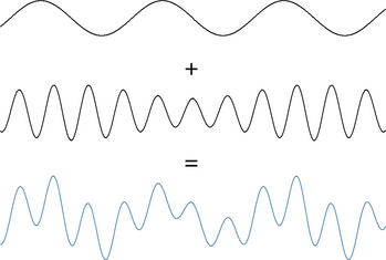
One important skill in EEG interpretation is the ability to “deconstruct” EEG waves visually into their component frequencies. The idea that a repetitive complex wave can always be broken down into simpler, fundamental waves was proved by Joseph Fourier in a mathematical theorem called the Fourier theorem. This theorem states, in simplified terms, that any waveform, no matter how simple or complex, can be exactly described by the sum of a sufficient number of simple sine waves. Although a comprehensive discussion of the Fourier theorem is beyond the scope of this text and not necessary to EEG interpretation, it reminds us that even the most complex EEG waves may be thought of as the sum of some number of fundamental sine waves. For example, the apparent complex wave shown in Figure 3-5 actually represents the combination of a 1-Hz wave, a 2.4-Hz wave, an 11.7-Hz wave, and a 34-Hz wave, each of a different amplitude. It is not necessarily the electroencephalographer’s goal to identify all of the component parts of any particular EEG wave, but it is useful to be able to identify the fundamental wave and the main superimposed waves of an EEG signal. Figures 3-6 through 3-9 illustrate the component waves that make up the complex wave of this example.

Figure 3-5 The complex waveform shown in this figure represents the summation of four separate sine waves with frequencies of 1 Hz, 2.4 Hz, 11.7 Hz, and 34 Hz wave, each of a different amplitude. The four individual contributing components of the wave are shown in the following figures. A 1-second scale is shown.

Figure 3-6 The original 1-Hz component of the mixed wave is superimposed on it. Some of the gradual “up and down” shape of the complex wave can be seen to be explained by this underlying 1-Hz slow-wave component, but the contribution of this slow component is difficult to visualize.

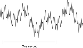
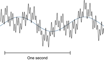
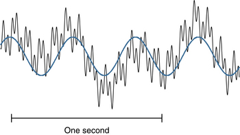
Figure 3-7 The same wave as Figure 3-6 with the 2.4-Hz component isolated and superimposed. Of all the component waves (with the possible exception of the fastest 34-Hz wave), this 2.4-Hz component frequency can be most easily identified in the mixed wave. Along with the 1-Hz wave, the 2.4-Hz wave lends some of the “roller-coaster” shape to the final wave.

Figure 3-8 The 11.7-Hz wave component is shown above the mixed wave for the sake of clarity. This specific component is somewhat difficult for the eye to sort out from the mixture of frequencies in the complex wave, but it can be identified.

Figure 3-9 The 34-Hz component of the initial wave is probably the easiest to identify. It is seen to “ride” atop the lower frequency waves.

For those interested in the basic mathematics that describe these waves, a review of the formula for a simple sine wave function helps us to recall some of the features of a wave that can be described thus:

In this formula, varying the coefficient A higher and lower will change the height or amplitude of the resulting wave. Varying b will change the frequency of the wave. Finally, changing the value of φ will shift the wave to the left or right on the x axis, which is also referred to as shifting the phase of the wave. It is not necessary to know this formula to interpret EEGs, but it is useful to keep the formula and its coefficients in mind when learning to separate out and describe the component parts of wave mixtures.

Although addition of one sine wave to another can be described with mathematical formulas, it is more useful to become accustomed to the appearance of how sine waves add visually as opposed to mathematically.

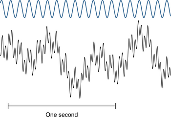
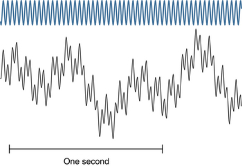
Figure 3-10 shows the result of superimposing or adding a lower voltage 10-Hz wave onto a higher voltage 1-Hz wave. Note that the lower voltage fast activity appears to “ride” the hills and valleys of the slower wave. The key is that both individual waves can still be visually appreciated even though they are mixed together.

Figure 3-10 The result of the addition of a 1-Hz wave to a lower voltage 10-Hz wave is shown. The top trace shows a 1-Hz sine wave at an amplitude of 100 μV, and the middle trace shows a 10-Hz wave at 20 μV. When the 1-Hz and 10-Hz waves are added together, the bottom wave results, showing the 10-Hz wave “riding” on the fundamental 1-Hz frequency.

When two waves are mixed and one has a frequency that is a multiple of the other, the higher frequency multiple is called a harmonic, and the lower frequency wave may be called the fundamental frequency. (Occasionally, the lower frequency wave may be called the subharmonic.) For instance, if there is a 5-Hz fundamental frequency, it is not uncommon to see a superimposed 10-Hz harmonic. When a wave is mixed together with its harmonic, the resulting wave often has a particular appearance of regular notching.

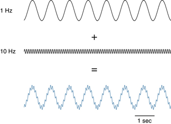
Figure 3-11 shows an example of adding a 2-Hz wave to its 4-Hz harmonic. Note how the shoulder of the slower wave is regularly notched by the faster wave in this idealized example. The notching may appear on the upslope, downslope, peak, or trough of the slower wave, depending on how the phase of one wave is lined up with the phase of the other when the two are added together. This pattern is important to recognize because the notching patterns created by these harmonics can occasionally be mistaken for spike-wave discharges.

Figure 3-11 This figure illustrates the addition of a fundamental wave to its harmonic. The top trace shows the fundamental 2-Hz wave at 25 μV, and the middle trace shows a 4-Hz sine wave of the same amplitude. When a wave is added to another wave that is a multiple of the first wave’s frequency (i.e., a harmonic frequency), the distinctive tracing seen in the bottom trace results. Note the regular “notching” pattern of the smaller wavelet riding on the larger wave. Because the two waves partially reinforce, the summation wave has an amplitude of 40 μV in this example. The degree to which the two waves reinforce and the particular shape that results is partly a function of how the two waves are shifted in the left–right axis with regard to one another (phase shift).

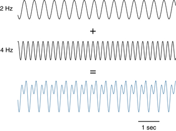
Figure 3-12 shows how the appearance of the superimposition of the same 2-Hz and 4-Hz waveforms can differ depending on how the phase of one is shifted to the right or left in comparison to the other.

Figure 3-12 The two waves shown here represent the summation of the exact same two component waves (top and middle waves) from the previous figure, except that the phase of the second wave is shifted to the left or right a slightly different amount compared with the first wave before the two are added together. Such combinations of fundamental waves with their harmonics do occur in cortical circuits and should not be mistaken for “spike wave.”

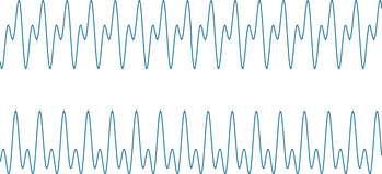
Figure 3-13 shows the result of adding a fundamental 2-Hz wave (top trace) to a 7-Hz wave of slightly varying amplitude (middle trace). In reality, the important skill is not necessarily to be able to predict what the result will be of adding two particular waves together but, rather, the reverse procedure: to be able to look at the bottom trace in Figure 3-13 and to be able to visually reconstruct the distinct 2-Hz and 7-Hz rhythms contained within the more complex waveform. Although the examples shown in these figures are of idealized sine waves, the same visual skills apply to the “deconstruction” of actual EEG waveforms. Of course, the idealized waves seen in these examples do not occur in such pure forms in complex biological systems such as the brain, which are more complex and subject to more variation.

Figure 3-13 The top trace shows a 2-Hz wave of constant amplitude, and the middle trace shows a 7-Hz wave of slightly varying amplitude. The bottom wave shows the result of adding the top wave to the middle wave. In this example, the 7-Hz activity is most readily appreciated in the combined wave, whereas the 2-Hz component is less obvious, although it makes a definite contribution to the final wave’s shape.

Figures 3-14 and 3-15 show examples of other ways that pure sine waves can vary, such as in frequency and amplitude, and represent somewhat more realistic approximations of real-life EEG waves.

Figure 3-14 The sine wave shown has a constant amplitude (height) but a 15% variation in frequency. Note that the width of each wave increases and decreases perceptibly. Such slight variations in frequency are common in physiologic EEG waves.

Figure 3-15 This sine wave has the same average frequency as the previous wave, but in this example, the frequency is held constant, and there is a 10% variation in the wave’s amplitude.

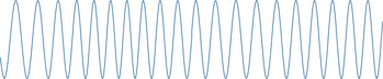
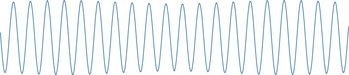
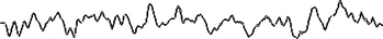
Figure 3-16 shows a close-up of a recorded EEG wave that contains mixed frequencies.

Figure 3-16 An EEG signal acquired from a patient shows a complex, “real-world” mixture of delta, theta, and faster rhythms. Although some sinusoidal elements can be appreciated, many of the waveforms are irregular.

Related posts:

The Structure and Philosophy of the EEG Report Introduction EEG Patterns in Stupor and Coma Electroencephalographic Electrodes, Channels, and Montages and How They Are Chosen The Abnormal EEG Filters in the Electroencephalogram

Stay updated, free articles. Join our Telegram channel

Join