3 Basic Nerve Conduction Studies
Peripheral nerves usually can be easily stimulated and brought to action potential with a brief electrical pulse applied to the overlying skin. Techniques have been described for studying most peripheral nerves. In the upper extremity, the median, ulnar, and radial nerves are the most easily studied; in the lower extremity, the peroneal, tibial, and sural nerves are the most easily studied (see Chapters 10 and 11). Of course, the nerves selected for study depend on the patient’s symptoms and signs and the differential diagnosis. Motor, sensory, or mixed nerve studies can be performed by stimulating the nerve and placing the recording electrodes over a distal muscle, a cutaneous sensory nerve, or the entire mixed nerve, respectively. The findings from motor, sensory, and mixed nerve studies often complement one another, and yield different types of information based on distinct patterns of abnormalities, depending on the underlying pathology.
Motor Conduction Studies
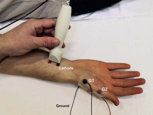
Motor responses typically are in the range of several millivolts (mV), as opposed to sensory and mixed nerve responses, which are in the microvolt (µV) range. Thus, motor responses are less affected by electrical noise and other technical factors. For motor conduction studies, the gain usually is set at 2 to 5 mV per division. Recording electrodes are placed over the muscle of interest. In general, the belly–tendon montage is used. The active recording electrode (also known as G1) is placed on the center of the muscle belly (over the motor endplate), and the reference electrode (also known as G2) is placed distally, over the tendon to the muscle (Figure 3–1). The designations G1 and G2 remain in the EMG vernacular, referring to a time when electrodes were attached to grids (hence the G) of an oscilloscope. The stimulator then is placed over the nerve that supplies the muscle, with the cathode placed closest to the recording electrode. It is helpful to remember “black to black,” indicating that the black electrode of the stimulator (the cathode) should be facing the black recording electrode (the active recording electrode). For motor studies, the duration of the electrical pulse usually is set to 200 ms. Most normal nerves require a current in the range of 20 to 50 mA to achieve supramaximal stimulation. As current is slowly increased from a baseline 0 mA, usually by 5 to 10 mA increments, more of the underlying nerve fibers are brought to action potential, and subsequently more muscle fiber action potentials are generated. The recorded potential, known as the compound muscle action potential (CMAP), represents the summation of all underlying individual muscle fiber action potentials. When the current is increased to the point that the CMAP no longer increases in size, one presumes that all nerve fibers have been excited and that supramaximal stimulation has been achieved. The current is then increased by another 20% to ensure supramaximal stimulation.
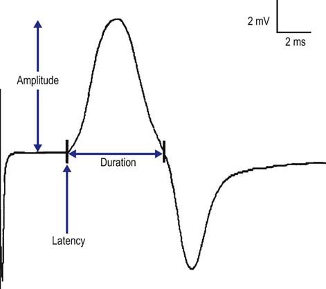
The CMAP is a biphasic potential with an initial negativity, or upward deflection from the baseline, if the recording electrodes have been properly placed with G1 over the motor endplate. For each stimulation site, the latency, amplitude, duration, and area of the CMAP are measured (Figure 3–2). A motor conduction velocity can be calculated after two sites, one distal and one proximal, have been stimulated.
Area
CMAP area also is conventionally measured as the area above the baseline to the negative peak. Although the area cannot be determined manually, the calculation is readily performed by most modern computerized EMG machines. Negative peak CMAP area is another measure reflecting the number of muscle fibers that depolarize. Differences in CMAP area between distal and proximal stimulation sites take on special significance in the determination of conduction block from a demyelinating lesion (see section on Conduction Block).
Conduction Velocity
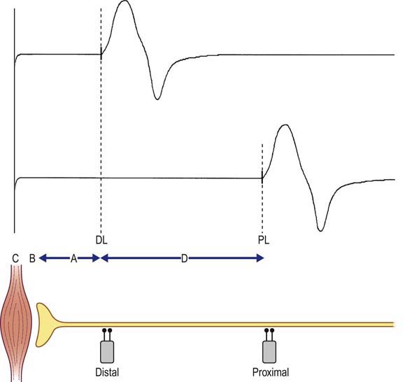
When the nerve is stimulated proximally, the resulting CMAP area, amplitude, and duration are, in general, similar to those of the distal stimulation waveform. The only major difference between CMAPs produced by proximal and distal stimulations is the latency. The proximal latency is longer than the distal latency, reflecting the longer time and distance needed for the action potential to travel. The proximal motor latency reflects four separate times, as opposed to the three components reflected in the distal motor latency measurement. In addition to (A) the nerve conduction time between the distal site and the NMJ, (B) the NMJ transmission time, and (C) the muscle depolarization time, the proximal motor latency also includes (D) the nerve conduction time between the proximal and distal stimulation sites (Figure 3–3). Therefore, if the distal motor latency (containing components A + B + C) is subtracted from the proximal motor latency (containing components A + B + C + D), the first three components will cancel out. This leaves only component D, the nerve conduction time between the proximal and distal stimulation sites, without the distal nerve conduction, NMJ transmission, and muscle depolarization times. The distance between these two sites can be approximated by measuring the surface distance with a tape measure. A conduction velocity then can be calculated along this segment: (distance between the proximal and distal stimulation sites) divided by (proximal latency − distal latency). Conduction velocities usually are measured in meters per second (m/s).
Sensory Conduction Studies
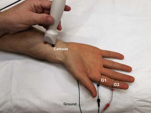
In contrast to motor conduction studies, in which the CMAP reflects conduction along motor nerve, NMJ, and muscle fibers, in sensory conduction studies only nerve fibers are assessed. Because most sensory responses are very small (usually in the range of 1 to 50 µV), technical factors and electrical noise assume more importance. For sensory conduction studies, the gain usually is set at 10 to 20 µV per division. A pair of recording electrodes (G1 and G2) are placed in line over the nerve being studied, at an interelectrode distance of 2.5 to 4 cm, with the active electrode (G1) placed closest to the stimulator. Recording ring electrodes are conventionally used to test the sensory nerves in the fingers (Figure 3–4). For sensory studies, an electrical pulse of either 100 or 200 ms in duration is used, and most normal sensory nerves require a current in the range of 5 to 30 mA to achieve supramaximal stimulation. This is less current than what is usually required for motor conduction studies. Thus, sensory fibers usually have a lower threshold to stimulation than do motor fibers. This can easily be demonstrated on yourself; when slowly increasing the stimulus intensity, you will feel the paresthesias (sensory) before you feel or see the muscle start to twitch (motor). As in motor studies, the current is slowly increased from a baseline of 0 mA, usually in 3 to 5 mA increments, until the recorded sensory potential is maximized. This potential, the sensory nerve action potential (SNAP), is a compound potential that represents the summation of all the individual sensory fiber action potentials. SNAPs usually are biphasic or triphasic potentials. For each stimulation site, the onset latency, peak latency, duration, and amplitude are measured (Figure 3–5). Unlike motor studies, a sensory conduction velocity can be calculated with one stimulation site alone, by taking the measured distance between the stimulator and active recording electrode and dividing by the onset latency. No NMJ or muscle time needs to be subtracted out by using two stimulation sites.
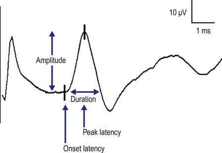
Peak Latency
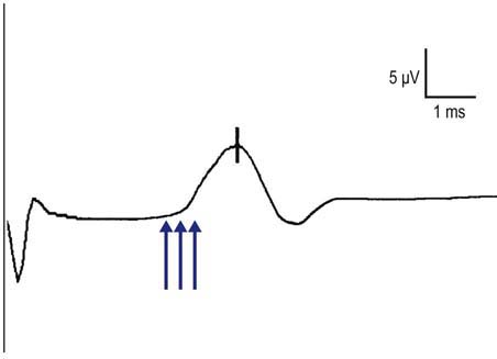
The peak latency is measured at the midpoint of the first negative peak. Although the population of sensory fibers represented by the peak latency is not known (in contrast to the onset latency, which represents the fastest conducting fibers in the nerve being studied), measurement of peak latency has several advantages. The peak latency can be ascertained in a straightforward manner; there is practically no interindividual variation in its determination. In contrast, the onset latency can be obscured by noise or by the stimulus artifact, making it difficult to determine precisely. In addition, for some potentials, especially small ones, it may be difficult to determine the precise point of deflection from baseline (Figure 3–6). These problems do not occur in marking the peak latency. Normal values exist for peak latencies for the most commonly performed sensory studies stimulated at a standard distance. Note that the peak latency cannot be used to calculate a conduction velocity.
Duration
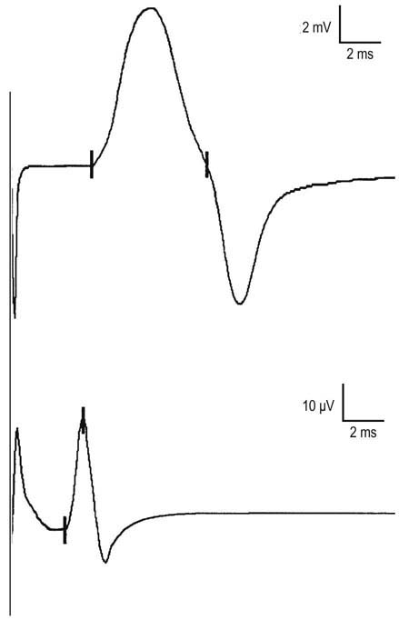
Similar to the CMAP duration, SNAP duration is usually measured from the onset of the potential to the first baseline crossing (i.e., negative peak duration), but it also can be measured from the initial to the terminal deflection back to baseline. The former is preferred given that the SNAP duration measured from the initial to terminal deflection back to baseline is difficult to mark precisely, because the terminal SNAP returns to baseline very slowly. The SNAP duration typically is much shorter than the CMAP duration (typically 1.5 vs. 5–6 ms, respectively). Thus, duration is often a useful parameter to help identify a potential as a true nerve potential rather than a muscle potential (Figure 3–7).
Special Considerations in Sensory Conduction Studies: Antidromic versus Orthodromic Recording
When a nerve is depolarized, conduction occurs equally well in both directions away from the stimulation site. Consequently, sensory conduction studies may be performed using either antidromic (stimulating toward the sensory receptor) or orthodromic (stimulating away from the sensory receptor) techniques. For instance, when studying median sensory fibers to the index finger, one can stimulate the median nerve at the wrist and record the potential with ring electrodes over the index finger (antidromic study). Conversely, the same ring electrodes can be used for stimulation, and the potential recorded over the median nerve at the wrist (orthodromic study). Latencies and conduction velocities should be identical with either method (Figure 3–8), although the amplitude generally is higher in antidromically conducted potentials.
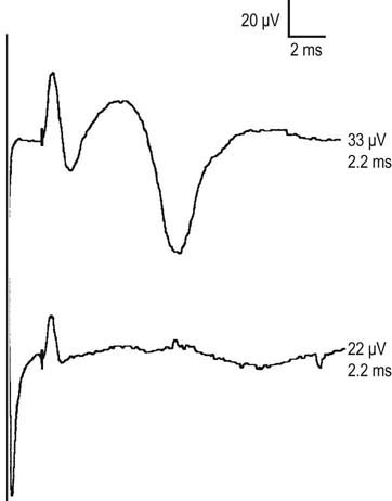
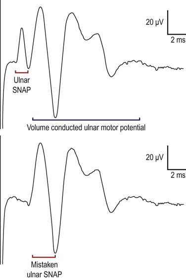
However, the antidromic method has some disadvantages (Figure 3–9). Since the entire nerve is often stimulated, including the motor fibers, this frequently results in the SNAP being followed by a volume-conducted motor potential. It usually is not difficult to differentiate between the two, because the SNAP latency typically occurs earlier than the volume-conducted motor potential. However, problems occur if the two potentials have a similar latency or, more importantly, if the sensory potential is absent. When the latter occurs, one can mistake the first component of the volume conducted motor potential for the SNAP, where none truly exists. It is in this situation that measuring the duration of the potential can be helpful in distinguishing a sensory from a motor potential. If one is still not sure, performing an orthodromic study will settle the issue, as no volume conducted motor response will occur with an orthodromic study. In this case, the antidromic and orthodromic potentials should have the same onset latency.

Stay updated, free articles. Join our Telegram channel

Full access? Get Clinical Tree


