Biophysical Aspects of EEG and Magnetoencephalogram Generation
Fernando H. Lopes Da Silva
Ab Van Rotterdam
The electrical activity of the brain consists of ionic currents generated by biochemical sources at the cellular level. These ionic currents cause electric and magnetic fields that can be measured in the brain and surrounding tissues. The behavior of these fields can be predicted because they obey physical laws. This chapter is an introduction to the biophysical aspects of the generation of electroencephalogram (EEG) signals. It is convenient to consider the generation of EEG signals in biophysical terms because this is the exact way to determine the potential distribution at the scalp given a set of intracerebral current sources, that is, the so-called forward problem of electroencephalography. An understanding of this problem is necessary to discuss the inverse problem that constitutes the main concern of clinical electroencephalography, which is to determine the intracerebral sources given a measured potential distribution at the scalp. The inverse problem has no unique solution, as shown long ago by Helmholtz (1); therefore, it is essential to understand the forward problem so that constraints of the inverse problem may be well examined.
This chapter treats the biophysical basis of the generation of EEG potentials nonmathematically so that the general reader may follow it more easily; in the theoretical appendix, a mathematical treatment of the biophysical aspects is provided.
SPACE-DEPENDENT PROPERTIES
The electrical potential at a point in the brain in principle can be computed if the microscopic cellular sources are known. In expression 5.8 of the Appendix, the field potential is given as a function of intracerebral current sources; in expression 5.10, it is given in terms of the membrane potential.
In general terms, the field potential of a population of neurons equals the sum of the field potentials of the individual neurons. To understand EEG phenomena, the activity of populations of neurons must always be considered. EEG phenomena can be measured only at a considerable distance from the source if the responsible neurons are regularly arranged and activated in a more or less synchronous way. A typical regular arrangement is the palisade, in which the neurons are distributed with the main axes of the dendritic trees parallel to each other and perpendicular to the cortical surface. When in such a population (e.g., the pyramidal neurons of layers IV and V of the cortex) the neurons are more or less simultaneously activated by way of synapses lying at the proximal dendrites, extracellular currents will flow; their longitudinal components (i.e., parallel to the main axes of the neurons) will add, whereas their transverse components will tend to cancel out. The result is a laminar current along the main axes of the neurons. The net membrane current that results from the activation at the level of the synapse can be either a positive or a negative ionic current directed to the inside of the cell. Because there is no accumulation of charge anywhere in the medium (see also Appendix, expression 5.1), the injected current at the synaptic level is compensated by other currents flowing in the medium, as shown in Figure 5.1. At the level of the synapse and in the case of an excitatory postsynaptic potential (EPSP), the synaptic current is carried by positive ions; in the case of an inhibitory postsynaptic potential (IPSP), the corresponding current is carried by negative ions. Because the direction of a current is defined by the direction along which the positive charge is
transported, the ionic current is directed to the intracellular medium with an EPSP; with an IPSP, it is directed to the extracellular medium. Therefore, at the level of the synapse, there is an active sink in the case of a positive ionic current (EPSP) or an active source in the case of a negative ionic current (IPSP). The extracellular potential at the sink is negative; at the source, it is positive, as can be seen from expression 5.8. Along the cell and at a distance from the synaptic level, there exists a distributed passive source in the case of an EPSP or a distributed passive sink in the case of an IPSP.
transported, the ionic current is directed to the intracellular medium with an EPSP; with an IPSP, it is directed to the extracellular medium. Therefore, at the level of the synapse, there is an active sink in the case of a positive ionic current (EPSP) or an active source in the case of a negative ionic current (IPSP). The extracellular potential at the sink is negative; at the source, it is positive, as can be seen from expression 5.8. Along the cell and at a distance from the synaptic level, there exists a distributed passive source in the case of an EPSP or a distributed passive sink in the case of an IPSP.
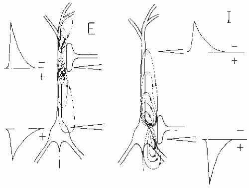 Figure 5.1 Current flow patterns in and around an idealized neuron owing to synaptic activation. E, current flow caused by activation of a synapse at the level of the apical dendrite resulting in depolarization of the membrane and flow of a net positive current. This current causes a sink at the site of the synapse. The extracellularly measured excitatory postsynaptic potential (EPSP) is drawn at the left; it has a negative polarity at the level of the synapse. At the soma there exists a distributed passive source resulting in an extracellular potential of positive polarity. I, current flow caused by activation of a synapse at the level of the soma resulting in hyperpolarization of the membrane and flow of a net negative current. This results in an active source at the level of the soma and passive sinks at the basal and distal dendrites. The extracellularly measured inhibitory postsynaptic potentials (IPSPs) at the soma and dendritic level are drawn. Note that an inhibition at the soma generates about the same extracellular potential field as an excitation at the apical or distal dendrites. |
In addition to postsynaptic potentials, other relatively slow variations of membrane potential, such as those associated with depolarizing or hyperpolarizing afterpotentials and dendritic events as calcium action potentials, may also be the sources of extracellularly measurable potentials.
At a macroscopic level, it may therefore be stated that the potential field generated by a synchronously activated palisade of neurons behaves like that of a dipole layer. This is no more than a rough model of reality. It may also be considered that an active sink (for instance, at the level of the cell somata in the cortex) is flanked by two passive sources, one lying more superficially and the other deeper than the sink; in such a case, the potential field should behave more like a quadrupole layer. This is, however, an unnecessary complication because in general the two sides of the quadrupole are rather asymmetrical; one is usually dominant. This is to be expected because it can be seen from histological sections of the cortex that there is a clear asymmetry of the pyramidal cells along a direction perpendicular to the cortex. These cells present a morphological polarization in the vertical direction because they are characterized by a rather long vertically directed apical dendrite that ramifies in the most superficial layers of the cortex and by basal dendrites distributed around the soma; the axon runs vertically downward to the white matter. For the sake of simplicity, it therefore may be assumed that most potential fields generated in palisades of neurons can be mimicked by simple dipole layers. Lorente de No (2) named this type of potential field the “open field” (Fig. 5.2C) (3), in contrast to those fields generated by neurons with dendritic arborizations radially distributed about the soma; according to his description, these would generate “closed fields” as shown in Figure 5.2A,B. In the latter case, the configuration of the radially oriented neurons is such that each neuron may be considered as generating a central source (or sink, depending on the type of synaptic activity) surrounded by spherically distributed sinks (or sources). The field potential in this case is equivalent to that of a distribution of radially oriented dipoles at the surface of a sphere. It can be seen intuitively that, under these circumstances, not only the tangential but also the radial components of current cancel each other; this can also be proved by the volume conduction theory (Fig. 5.3) (4).
Postsynaptic potentials in neuronal populations with an appropriate spatial organization can be sources of field potentials that can be measured at a distance and therefore are also sources of EEG signals. Can other types of membrane potentials as action potentials also contribute to those EEG signals? This is not generally the case for two reasons (see also Appendix). The first reason is that the membrane potential variation caused by an action potential generates a field that is equivalent to that of a single dipole perpendicular to the membrane because the piece of membrane that is depolarized at any instant of time is small. In contrast, that of an electrotonically conducted postsynaptic potential extends, at any moment of time, over a larger portion of the membrane; thus, it generates a field that corresponds rather to that of a dipole layer with dipoles perpendicular to the membrane surface. The latter
attenuates with distance less rapidly than the former, as can be seen by comparing expressions 5.12 and 5.15 of the Appendix; this is illustrated in Figure 5.10B and has also been discussed by Humphrey (5). These properties have been analyzed more rigorously by Pettersen and Einevoll (6) using realistic computer models of pyramidal and stellate neurons with different morphologies. These authors demonstrated that the neural morphology and passive electrical parameters influence the width and amplitude of extracellular spikes. These modeling studies revealed that in all neurons there is a low-pass filtering effect, that is, the spike-width increases with increasing distance from soma. These authors showed quantitatively that the spike-amplitude decays with distance r depending on dendritic morphology, according to the rule 1/rn with 1 ≤ n ≤ 2 close to the soma and n ≥ 2 far away along the dendritic tree. These studies have also implications for understanding the relation between the extent of fields produced by multiunit activity (MUA) and by synaptic potentials, which constitute the so-called local field potentials (LFPs or local EEG), since they substantiate why MUAs are more confined around the neural sources than the LFPs generated by synaptic currents. In the latter case the dipole layer lengths are much longer than the typical action-potential current dipoles, and thus the attenuation with distance is weaker than for the MUAs. The second reason that action potentials do not contribute to EEG signals is that the latter, owing to their short duration (1 to 2 msec), tend to overlap much less than do postsynaptic potentials (EPSP and IPSP), which last longer (10 to 250 msec). In those cases in which the action potentials occur simultaneously in clusters (e.g., when a group of fibers is excited by a short stimulus), the field of these action potentials may also be recorded at relatively large distances in the form of what is generally called a “compound action potential.”
attenuates with distance less rapidly than the former, as can be seen by comparing expressions 5.12 and 5.15 of the Appendix; this is illustrated in Figure 5.10B and has also been discussed by Humphrey (5). These properties have been analyzed more rigorously by Pettersen and Einevoll (6) using realistic computer models of pyramidal and stellate neurons with different morphologies. These authors demonstrated that the neural morphology and passive electrical parameters influence the width and amplitude of extracellular spikes. These modeling studies revealed that in all neurons there is a low-pass filtering effect, that is, the spike-width increases with increasing distance from soma. These authors showed quantitatively that the spike-amplitude decays with distance r depending on dendritic morphology, according to the rule 1/rn with 1 ≤ n ≤ 2 close to the soma and n ≥ 2 far away along the dendritic tree. These studies have also implications for understanding the relation between the extent of fields produced by multiunit activity (MUA) and by synaptic potentials, which constitute the so-called local field potentials (LFPs or local EEG), since they substantiate why MUAs are more confined around the neural sources than the LFPs generated by synaptic currents. In the latter case the dipole layer lengths are much longer than the typical action-potential current dipoles, and thus the attenuation with distance is weaker than for the MUAs. The second reason that action potentials do not contribute to EEG signals is that the latter, owing to their short duration (1 to 2 msec), tend to overlap much less than do postsynaptic potentials (EPSP and IPSP), which last longer (10 to 250 msec). In those cases in which the action potentials occur simultaneously in clusters (e.g., when a group of fibers is excited by a short stimulus), the field of these action potentials may also be recorded at relatively large distances in the form of what is generally called a “compound action potential.”
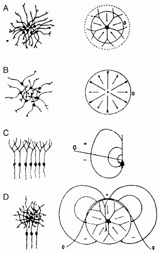 Figure 5.2 Examples of closed, open, and open-closed fields for different types of neuron pools in the central nervous system. Left: The populations are drawn. Right: Neurons representing the simultaneously activated pools are shown together with the arrows representing the lines of flow of current at the instant when the impulses have evaded the cell bodies. The zero isopotential lines (0) are also indicated. A: Oculomotor nucleus represented schematically by only one neuron with dendrites oriented radially outward. The isopotential lines are circles; the currents flow entirely within the nucleus, resulting in closed field (all points outside the nucleus remain at zero potential). B: Superior olive represented by neurons each having a single dendrite oriented radially inward. The currents result in a closed field. C: Accessory olive represented by only one neuron with a single long dendrite. The arrangement of sources and sinks in this structure permits the spread of current in the volume of the brain and thus results in an open field. D: Two structures mixed together, generating an open-closed field. (Modified from Lorente de No R Action potential of the motoneurons of the hypoglossus nucleus. J Cell Comp Physiol. 1947;29: 207-287; Hubbard, J I, Llinas, R Quastel D M J Electrophysiological Analysis of Synaptic Transmission. London: Edward Arnold Ltd; 1969.) |
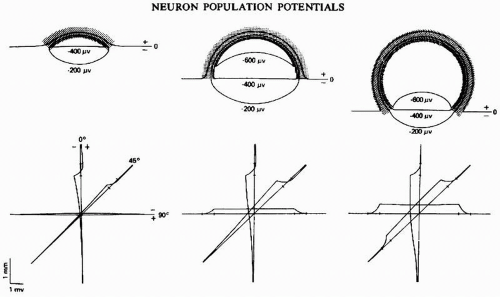 Figure 5.3 Equipotential plots and depth profiles for open cortices. Intersection of base lines of the depth profiles is at the center of the sphere. Tick marks represent the region of cells. Note that the 90-degree profile of the hemisphere and 45-degree profiles of the cap and punctured sphere run along the open edge of the cortex. (Adapted from Klee M, Rall W. Computed potentials of cortically arranged populations of neurons. J Neurophysiol. 1977;40:647-666.) |
Quantitative measurements in vitro and computational neuronal models used to infer contributions of neuronal populations to MEG and EEG signals.
Studies using in vitro preparations allow the simultaneous measurement of electric and magnetic fields generated by neuronal activity. A calculation of the magnetic field around an axon was performed by Swinney and Wikswo (7) using a preparation where an isolated axon was kept in a bath with saline, in vitro, and was stimulated electrically. These authors found that the magnetic field resulted mainly from the intracellular current flowing inside the axon along the axial direction, whereas the contribution of the return passive current that flows in the medium was two orders of magnitude smaller, and that of the transmembrane current was negligible.
More recently, Murakami and Okada (8) applied the same kind of approach to the neocortex. This study is particularly relevant because it has yielded some results that may help to interpret EEG and magnetoencephalogram (MEG) recordings from the scalp. These authors made a computer model, based on that proposed by Mainen and Sejnowski (9), of the four main types of cortical neurons taking into account their realistic shapes. Each neuron is described as a three-dimensional
compartmental model, where each compartment has its typical geometric dimensions, passive electrical properties (membrane capacitance and resistance, intracellular resistance), and five voltage-dependent ionic conductances. Neuronal activity was obtained by stimulating each neuron with an intracellular current injected at the soma. The intracellular current is represented by a vector quantity, the magnitude of which is the current dipole moment and is represented by the scalar quantity Q in [pA m].
compartmental model, where each compartment has its typical geometric dimensions, passive electrical properties (membrane capacitance and resistance, intracellular resistance), and five voltage-dependent ionic conductances. Neuronal activity was obtained by stimulating each neuron with an intracellular current injected at the soma. The intracellular current is represented by a vector quantity, the magnitude of which is the current dipole moment and is represented by the scalar quantity Q in [pA m].
The population Q for a group of pyramidal neurons was calculated by computing the sum of the dot product of each current dipole Qk and the unit vector orthogonal to the cortical surface. The same was done for the stellate cells, with a modification due to the fact that these neurons are differently oriented. The magnetic field B and electrical potential V at the scalp can be expressed as functions of the intracellular currents, called primary currents, and the return currents that flow in the space around the sources. In the model the magnetic field B is assumed to be generated by the tangential component of Q, with respect to the inner skull surface, and the electric field is due to both the tangential and radial components. This implies that B is mainly caused by neuronal activity in sulci, since Q is directed perpendicularly to the pial surface, whereas both radial and tangential components contribute to the electric field. This investigation led to another result of practical interest, namely it gave some direct indications about how to interpret the magnitude of the magnetic fields recorded in human. According to the model the overall magnitude of Q for the activity of pyramidal neurons of layers V and II/III is in the order of 0.29 to 0.90 pA m. Apparently this value deviates appreciably from that estimated previously for a cell by Hämäläinen et al. (10) that was just 0.02 pA m. That larger value, however, is of the same order of magnitude as those estimated for hippocampal pyramidal neurons (0.2 pA m per cell in CA1 and 0.17 pA m per cell in CA3, (11,12)). Murakami and Okada (8) point out that assuming a Q of 0.2 pA m per cortical pyramidal neuron, a population of 50,000 synchronously active cells would generate a field with a magnitude of 10 nA m, which corresponds precisely to the smallest value measurable from the human cortex according to Hämäläinen et al. (10). Assuming that a cortical minicolumn with a diameter of 40 µm contains 100 cells (13), the cortical surface that would correspond to 50,000 cells should form a patch with about 0.63 mm2 area. If this cortical patch would have a circular form its diameter would be about 0.9 mm.
In order to estimate the number of cortical cells corresponding to a cortical column, the synchronous activity of which is responsible for the EEG/MEG signal measured, one has to know, at least approximately, the density and the spatial distribution of pyramidal and other cell types within the cortex.
TIME-DEPENDENT PROPERTIES
We have emphasized above the importance of synchrony of neuronal activity for the generation of EEG signals. We consider here the factors that cause this synchrony. The main factor is of a structural nature. Neuronal masses are, in general, organized as combinations of interlocked excitatory and inhibitory populations (14, 15, 16, 17 and 18); the interlocking takes place by way of recurrent collaterals forming different types of synapses that possibly include dendrodendritic synapses and even gap junctions (19).
These neural masses act as macroscopic sources of EEG signals. For example, in the case of the generation of alpha rhythms, it has been shown that such a macroscopic source is located within the cortex and behaves like a dipole layer directed perpendicularly to the cortical surface (20). The dynamic properties of alpha rhythms, such as their frequency, depend on the parameters of the neuronal populations, such as feedback gains, strength of connections, time properties of synaptic potentials, and nonlinear properties (i.e., thresholds and saturation).
Does this rhythmic activity propagate along the cortex or form a standing field? It has been shown experimentally (20) that, in the visual cortex of the dog, small cortical areas appear to act as “epicenters” from which alpha rhythm activity “spreads” in different directions. The existence of this type of spread has been concluded on the basis of phase differences in rhythmic components measured at different locations on the cortical surface. It has been shown in a model study (21) that a neuronal chain, where the model neurons are interconnected by means of recurrent collaterals and interneurons such that the connectivity functions are homogeneous and their strength decays as an exponential function of distance, shows propagation of electrical activities characterized by frequencies in the alpha band with a velocity c in the order of magnitude of 0.3 m/sec, which is in the range of experimental results. The dynamics of the activity of neuronal populations are treated in more detail in Chapter 4.
The propagation of electric activity in the cortex may result in the interesting phenomenon of time dilation, that is, an EEG transient recorded at the cortex will seem to be of shorter duration than the transient recorded simultaneously at the scalp. This has been shown to occur in relation to epileptiform spikes (22). The phenomenon of time dilation is due to the fact that a moving dipole seen from a distance can be observed over a longer time than when seen from nearby. The physical basis for this phenomenon is accounted for in the Appendix (expression 5.18).
INFLUENCE OF INHOMOGENEITIES
It has been assumed that the brain could be considered an infinite homogeneous medium, but in reality this is not the case. The field potentials are influenced not only by the geometry of the neuronal populations and the electrical properties of individual neurons but also by the existence of regions with different conductivities in the head, that is, by the presence of inhomogeneities. For an interpretation of field potentials measured at the scalp, therefore, it is important to take into consideration the layers lying around the brain: the cerebrospinal fluid (CSF), the skull, and the scalp. These layers account, at least in part, for the attenuation of EEG signals measured at the scalp as compared to those recorded at the underlying cortical surface. This can be formulated in mathematical terms, as in the Appendix (expression 5.19).
To compute the potential distribution at the surface of the scalp caused by a dipole placed within the brain, it is necessary to compute the potential distribution at the surface of the different shells (i.e., to solve the boundary value problem). This can be done by solving the Poisson equation (see equation 5.7) in polar coordinates as done in the Appendix. Already in the 1970s, the influence on the EEG of the specific electrical properties of the tissues surrounding the brain was recognized (23, 24, 25, 26 and 27). The systematic study of Ary et al. (28) led to the proposal of a method that would correct the errors introduced by variations in skull and scalp thickness. Initially, the models of the head volume conductor consisted of concentric spheres, usually three to account for the brain, skull, and scalp; in some models a fourth layer was included representing the CSF. In the classic models, the three main concentric spheres typically had radii of 90, 83, and 78 mm. The values of the conductivities of the three layers commonly used were proposed by Geddes and Baker (29): for the brain 0.33, for the skull 0.0042, and for the scalp also 0.33 S.m-1; in case the CSF was included, it had a conductivity of 1.0 S.m-1. Recently more precise estimates of these conductivities were obtained by way of measurements in vivo, using an electric impedance tomography (EIT) method combined with a realistic model of the head (30, 31 and 32). The results of the study of Gonçalves et al. (32) showed that the ratio between the conductivities of the skull and the brain lies between 20 to 50 (for six subjects) rather than the traditionally assumed value of 80. The average values found in this investigation are the following: brain: 0.33 S.m-1; skull: 0.0081 S.m-1. It is also important to note that the intersubject variance of the estimates decreased by half when a realistic model was used, in comparison with a spherical model. However, a factor of 2.4 was found between the subjects with the extreme values of the ratio of conductivities. This implies that these values should be estimated for each individual to increase the reliability of the estimated conductivities.
In addition, it is known that the conductivity of the various tissues is not homogeneous. The conductivity of the skull varies with its thickness and bone structure. Law et al. (33) showed that there is an inverse relation between skull resistivity and thickness. Cuffin (34) and Eshel et al. (35) investigated the effects of varying the conductivity of the skull; the former determined that the effect of local variations in skull and scalp thickness was slightly larger on the EEG than on the MEG, while the latter showed a correlation between interhemispheric asymmetry in skull thickness and the amplitude of the scalp EEG. The very thorough studies of Haueisen (36,37) on the influence of various combinations of conductivities on both the EEG and MEG showed that the scalp EEG is most influenced by the conductivities of the skull and the scalp, while the MEG was most influenced by the conductivities of the brain tissue and the CSF. We should note that the conductivity of the tissues of the head can also present anisotropy. Indeed, it is known that in brain tissue, the conductivity measured in a direction parallel to a fiber tract can be 10 times larger than in the perpendicular direction (38). It is, however, difficult to integrate this finding in global models of the whole head, since fiber tracts are organized in a most complex way within the anatomical constraints of the folds of the brain. Nevertheless, De Munck (39), using a model consisting of five concentric shells, solved the forward problem in an analytic form for the case in which the skull and the cortex had anisotropic properties. The effects of the anisotropic conductivity of the skull were determined by Bertrand et al. (40) and by Van den Broek (41). The latter showed that the anisotropy of the skull causes the smearing out of the distribution of the EEG over the scalp, whereas the normal component of the MEG is not affected.
In addition, it is relevant to emphasize that the skull does not have a homogeneous surface, due to both the existence of regions with different thickness and the occipital and the eye sockets openings (42). The existence of holes in the skull, for example, due to surgical interventions, influences also the distribution of the EEG over the scalp as demonstrated by Bertrand et al. (40). In general, the localization of the dipoles is then shifted toward the hole.
REALISTIC MODELS OF THE HEAD AND NUMERICAL METHODS
In the past, most solutions of the forward problem assumed that the head could be reasonably approximated by a spherical model with three or four shells. However, the geometry of this volume conductor is clearly not spherical. Therefore, since the late 1980s, realistically shaped models were gradually introduced and applied (43, 44, 45, 46 and 47). This was made possible by the advances in magnetic resonance imaging (MRI) that allow making realistic estimates of the three-dimensional geometry of the brain and surrounding tissues (48). To solve the forward problem in a realistic shaped volume of the head, it is necessary to apply numerical methods. This involves decomposing the volume conductor in a mesh consisting of a relatively large number of discrete elements. The accuracy of the method increases with the number of these elements, and, of course, is inversely proportional to their size, but the computational effort also increases accordingly. The most commonly used methods to compute the EEG potential distributions are the boundary-element method (49, 50, 51, 52 and 53), which is appropriate to the case where the volume conductor is assumed to be isotropic and piecewise homogeneous, and the volume element methods, which are needed in case the assumptions of isotropy and piecewise homogeneity do not hold. Examples of the latter are the finite-volume (35), the finite-difference, and the finite-element methods (for details see reviews by van Uitert, Weinstein, and Johnson (54)). These methods are powerful, but they need reliable information about the structure of the brain and surrounding tissues, obtained from MRI scans, and of the corresponding conductivities, to be applied in a sensible way. They are particularly suited to calculate the influence of specific inhomogeneities such as the influence of the cerebral ventricles filled with CSF (41) and anisotropic conductivities (36).
In a number of studies, the advantage of using realistic models in comparison with spherical models has been demonstrated; differences in dipole reconstructions using EEG data were reported to reach 20 mm (55,56). Relatively smaller differences were obtained with MEG data, in the order of 4 mm (57). This implies that the necessity of using realistic models,
particularly those accommodating inhomogeneous volumes, is stronger for EEG than for MEG recordings. In the latter case, most calculations are based on the boundary-element method.
particularly those accommodating inhomogeneous volumes, is stronger for EEG than for MEG recordings. In the latter case, most calculations are based on the boundary-element method.
THE INVERSE PROBLEM: APPROACHES TO ESTIMATE SOLUTIONS
The introduction stated that the problem of calculating the intracerebral sources of the potentials measured at the scalp, that is, the so-called inverse problem of electroencephalography, has no unique solution. This means that different combinations of intracerebral sources can result in the same potential distribution at the scalp. The only way to tackle this problem is to make specific assumptions about the intracerebral sources that are assumed to cause a given EEG potential distribution and to make a model of the conductive media lying between the sources and the recording electrodes. This implies that first a particular type of forward problem is solved; thereafter, the theoretical scalp potentials obtained in this way are compared with those recorded experimentally. It should be noted that, on the one hand, a satisfactory comparison does not necessarily imply that the assumed sources are those really responsible for the measured EEG potentials. On the other hand, however, a bad comparison must lead to the conclusion that the assumptions are not correct with respect to the sources or to the model, or both.
The numerical procedures by means of which the measured EEG/MEG distribution over the scalp is compared with that computed using the forward approach are not trivial. Usually one expresses the difference between the real and the simulated distributions as a summed squared difference. The question is to find a minimum of this function, which can be accomplished by several algorithms. The mostly used of this is that of Marquardt (58). In the last decades many solutions of the inverse problem have been proposed, starting from the pioneer work of Schneider and Gerin (59), Schneider (25,26), Smith et al. (60), Henderson et al. (61), and many others as reviewed by Scherg (62,63) and Stok (64).
According to this approach, the intracerebral source is assumed to be an equivalent current dipole localized within the brain. Here we consider, in general terms, those aspects of the inverse problem that are common to EEG and MEG. The aim of the inverse procedure is to obtain an equivalent source, which in general is a dipole, determined by six parameters. This solution is called the equivalent dipole (ED), which must be considered a mathematical abstraction. It represents the theoretical dipole, which generates a potential (or magnetic field) distribution at the surface of the outer shell, that is the closest in the least square sense to the measured distribution at the scalp. It should be emphasized that the estimation of an ED located within the brain gives only a rough estimate of the center of gravity of the cortical area active at a given moment. For example, in the case of the dipole layer shown in Figure 5.3 the corresponding ED would be located much deeper than the surface where the individual dipolar sources are placed.
Assuming that the activity of each cortical macrocolumn would be described by an equivalent current dipole, one would need several thousands to account for an EEG or MEG scalp distribution. The number of sensors, however, is much smaller, in the order of a maximum of 128 for the EEG and 300 for the MEG. Thus, the problem of estimating brain sources of EEG or MEG data is underdetermined. Regularization methods have been proposed to help solve this major difficulty.
For solving the inverse problem, the method of the least-squares source estimation has been applied both to the activity measured at a single moment in time or within a time interval (65,66). In this context a convenient approach, proposed by De Munck (39,67), is to split the set of parameters of the ED into linear and nonlinear parameters. This procedure consists schematically of the following steps: first, the time functions that describe the change of the source as function of time must be estimated for a given position and orientation of the ED; second, the orientations must be found given the dipole time functions and position. These two steps must be performed alternatively a number of times until the best dipole orientation and time functions are found for given dipole positions. Thereafter, the nonlinear position parameters must be updated and the process repeated until a best fit is obtained. This procedure starts from the assumption that the position and orientation of the initial dipole are known, that is, it is based on the stationary dipole model proposed by Scherg and Von Cramon (65), although it is not constrained to the initial choice.
If a reasonable assumption on the initial position and orientation cannot be made, one may use the alternative approach of estimating EDs for a number of successive time samples of a given potential, or magnetic, distribution (so-called moving dipole approach) as done by Stok (64) and Stok et al. (68) and many others. In this way a series of EDs is obtained, as shown in Figure 5.4. Those EDs that have about the same position and orientation can be clustered and the clustered dipoles can be averaged. If desired, these average ED clusters can be used as seed points for the procedure of de Munck as described earlier (69).
We should note that, in practice, if the distribution of the EEG potential or of the MEG field over the scalp is relatively simple, a single ED may be an appropriate model. Of course, one needs all available a priori information to speed up the solution and to give it high reliability. For instance, if it is to be expected that a given activity occurs simultaneously in both hemispheres in areas well defined anatomically, it is advisable to start by assuming two symmetrical dipoles at the appropriate sites (63). An increase in the number of dipoles can easily lead to rather complex and ambiguous interpretations. Validation of ED models can be obtained in retrospect by relating the solutions obtained to independent physiological or anatomical information. An example of an anatomical-physiological validation is the case of the dipolar sources of alpha, mu rhythms, and sleep spindles (70) that are distributed on brain areas as expected on the basis of animal and human physiological observations. An example of anatomical-pathological validation is given by the distribution of sources of epileptiform transients in patients with cortical lesions visible in MRIs (Fig. 5.5), where the main epileptiform sources are located around the lesions (71,72).
A number of alternative methods have been developed to circumvent the obvious limitations of the ED approach. One of
these consists in applying spatial filtering to the data so that signals from a given location may be privileged with respect to the rest. This is the so-called linearly constrained minimum variance beam forming (73) that has been applied in practice with some interesting results (74). Related methods are the synthetic aperture magnetometry (SAM) method introduced by Robinson and Vrba (75), and the parametric mapping method applied by Dale et al. (76). In addition, methods have been proposed to obtain estimates of multiple dipoles with little a priori information, such as the multiple signal classification (MUSIC) algorithm (77, 78 and 79). A number of laboratories have pursued this issue by creating new algorithms based on the assumption that the sources are at fixed locations within the brain, namely at a given node of the triangular tessellation of the cortical surface as extracted from the subject’s MRI. In this way the inverse solution is simplified to finding the linear parameters of the sources. Nevertheless, this problem is still underdetermined. The methods used to solve this problem use different forms of regularization parameters (80). In this way particular forms of inverse solutions can be obtained: minimum norm (MN) (81, 82, 83 and 84), weighted resolution optimization (WROP) method of Grave de Peralta Menendez et al. (85), and the low-resolution
brain electromagnetic tomography (LORETA). The latter was proposed by Pascual-Marqui et al. (86) and uses the discrete spatial Laplacian operator for regularization. This method yields a very smooth inverse solution (87).
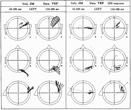 Figure 5.4 Projection of equivalent dipoles (EDs) based on visual evoked potentials (VEPs) (left) and visual evoked fields (VEFs) (right) during the on-response of subject JM, to the appearance of a checkerboard presented to the left half-visual field. Each ED is shown in three projection planes, namely occipital (top), horizontal (middle), and sagittal (bottom). An arrow indicates the direction and length of the projection of the dipole and the starting point indicates the dipole location. Each arrow is identified by a small number that runs from 1 to 11. A group of arrows represents an interval of 50 msec, in steps of 5 msec, spanning the time interval of 55 to 160 msec after start of the stimulus. Scale: one division indicates 10 mm for the position and 6.7 × 10⁻⁹ A m, for the components. Each dipole is plotted with a line width corresponding to the measure of fit χ2: thick for χ < 0.1, medium for 0.1 < χ < 0.2, thin for 0.2 < χ < 0.4, very thin for χ ≥ 0.4. (Modified from Stok CJ, Spekreijse HJ, Peters MJ, et al. A comparative EEG/MEG equivalent dipole study of the pattern onset visual response. New trends and advanced techniques in clinical neurophysiology. EEG Suppl. 1990;41:34-50.) |
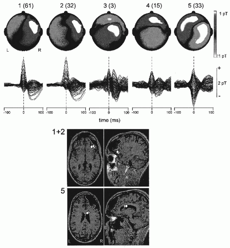 Figure 5.5 Top: Channel overlays and topographic maps of the average magnetic fields for the five spike clusters in patient C. The field maps represent the magnetic field distribution at the time of the marker, indicated in the channel overlays by the dashed vertical line. Above each map the cluster number and, within brackets, the number of spikes it contains. Bottom: Position of equivalent dipoles. In the top axial and sagittal magnetic resonance imaging (MRI) slices the dipoles fitted to the average magnetoencephalogram (MEG) spike of clusters 1 and 2, combined. In the bottom slices are the dipole locations for cluster 5. For clusters 3 and 4 equivalent dipole sources with less than 10% residual error were not found. The boundary of the structural lesion in the right frontal lobe for this patient is marked by dotted lines. (Adapted from Van’t Ent D, Manshanden I, Ossenblok P, et al. Spike cluster analysis in neocortical localization related epilepsy yields clinically significant equivalent source localization results in magnetoencephalogram [MEG]. Clin Neurophysiol. 2003;114(10):1948-1962.) |
In any case, dipole models provide less ambiguous solutions than the more sophisticated methods described above, since they are based on simpler assumptions. Nonetheless, they yield images that are less attractive than the latter methods. In any case, dipolar methods are only meaningful if the scalp field has approximately focal character.
Alternatively, the scalp EEG may be described using the surface Laplacian that estimates the local normal component of the current through the skull (33) and can be computed by applying either a local or a global approach. According to the local approach (88, 89 and 90), the surface Laplacian is computed locally using a subset of neighboring sensors for differentiation. According to the global approach (33,91,92), an interpolation function is first applied to the measurements obtained over the whole head and the differentiation is applied afterward. The relationship between the surface Laplacian and the cortical potential distribution is only simple in case of homogeneous skull and scalp layers. Zanow (93) compared, in a computer simulation study, the performance of the surface Laplacian and a linear estimation approach with dipoles having free moment orientations, the so-called cortical potential reconstruction based on linear estimation (Fig. 5.6). Compared to the surface Laplacian method, the latter linear estimation method provided a more accurate cortical image of the sources for a comprehensive review of these methodologies, see Ref. 94. Another alternative method consists in reconstructing the potential distribution on the inner boundary of the skull by the method of spatial deconvolution (89).
Related posts:
 Dynamics of EEGs as Signals of Neuronal Populations: Models and Theoretical Considerations
EEG of Degenerative Disorders of the Central Nervous System
Metabolic Disorders and EEG
Anticipating Seizures Based on EEG
Intracranial Monitoring: Depth, Subdural, and Foramen Ovale Electrodes
EEG Event-Related Desynchronization (ERD) and Event-Related Synchronization (ERS)
Dynamics of EEGs as Signals of Neuronal Populations: Models and Theoretical Considerations
EEG of Degenerative Disorders of the Central Nervous System
Metabolic Disorders and EEG
Anticipating Seizures Based on EEG
Intracranial Monitoring: Depth, Subdural, and Foramen Ovale Electrodes
EEG Event-Related Desynchronization (ERD) and Event-Related Synchronization (ERS)
Stay updated, free articles. Join our Telegram channel

Full access? Get Clinical Tree


