Dynamics of EEGs as Signals of Neuronal Populations: Models and Theoretical Considerations

Fernando H. Lopes Da Silva

MODELS OF EEG GENERATION—INTRODUCTION

In Chapters 2 and 3 the neurophysiological basis of the electroencephalogram (EEG) was discussed with special emphasis on the phenomena at the cellular level. In Chapter 5, the biophysical aspects of the generation of EEG phenomena are considered mainly in terms of volume conduction, but the dynamic properties of EEG patterns are only briefly mentioned. These dynamic properties, however, are essential for understanding EEG phenomena. In this chapter, EEG signals are considered as the result of the dynamic behavior of neuronal populations as revealed by model studies. According to this perspective, it is necessary to integrate experimental and theoretical results. The latter must be obtained using models of neuronal networks and corresponding computer simulations. The mathematical treatment of such models has been avoided here; the interested reader is referred to a number of other publications that are cited for their thorough mathematical treatment of these areas.

The fundamental assumption on which the following discussion is based is that EEG signals reflect the dynamics of electrical activity in populations of neurons. A property of such populations that is of utmost importance for the generation of EEG signals is the capacity of the neurons to work in synchrony. This depends on the connectivity between the neurons that form a network. The classic terminology of Freeman (1) provides a useful systematization. Populations of neurons with mutual interactions are called KI sets; the interactions may be excitatory (KIe) or inhibitory (KIi). Groups of two interacting populations of neurons are called KII sets; they are formed by an interaction of a KIe set with a KIt set. Further, KIII sets formed by the interaction between two KII sets can be defined. A number of such KIII sets constitute a neural mass that may occupy a few square millimeters of cortical surface or a few cubic millimeters of nuclear volume in the brainstem or spinal cord. Typically, a neural mass consists of approximately 10⁴ to 10⁷ neurons. An example of a KIII set is given in a symbolic way in Figure 4.1. An essential feature of such a basic module is the existence of multiple feedback loops. Such a set of neurons can produce oscillatory phenomena as revealed in EEG signals. The main parameters that characterize the dynamic behavior of the set are (a) the synaptic time constants; (b) the length constants, which define the distance of the interactions between different neurons; (c) the gain factors, that is, the strength of interactions, whether by way of chemical synapses or electrical couplings; and (d) the intrinsic ionic and synaptic currents.

There are both inhibitory and excitatory feedback loops. The terms negative feedback and positive feedback are often used in a rather loose way to characterize the interactions between populations of neurons. However, the sign of feedback is defined in an exact way by comparing the overall gain modulus of the system with feedback (closed loop gain: |Y_o(j)|) and without feedback (open loop gain: |Y₁(j)|). The feedback is said to be negative if |Y_o(j)| < |Y₁(j)| and positive in the opposite case (2). The exact sign of feedback in the interaction between neuron populations is in most cases not known. It therefore seems preferable to use the terms excitatory and inhibitory feedback to define the main synaptic type of interaction between neuron populations. This will be considered from the reference point of the “main” population, which usually is the population that receives the input from another source and/or sends its output to another structure.

In this chapter, models of the generation of characteristic types of EEGs, including the spatial spread of rhythmic activity over the cortex, and nonlinear dynamics as a new approach for understanding EEG phenomena are presented.

The processes of generation of EEG signals in a large number of neurons forming a neural mass are complex. Therefore, it is useful to use both analytic and synthetic approaches to understand such processes. It is essential to use both approaches in a dialectic way. The experimental data, obtained through histological and physiological analytic methods, must be put together just as pieces of a puzzle are assembled. Very often the relationship between the different pieces is still unclear. It is in this context that a synthetic approach may be most helpful. The point is then to put together the available data in such a way as to form the most likely pattern. In this way, a model of a neurophysiological system can be constructed. Such a model can help to advance knowledge of the system in two respects. First, it provides the possibility for testing the influence of different types of inputs or of changing some of the properties of the constituting elements upon the output of the system. Second, it allows the formulation of hypotheses concerning new elementary properties, relationships, and overall behavior; it may thus predict new properties of the system, raise new questions, and suggest new experiments to explore these hypotheses. In this way, the model can constitute a bridge between experimentation and theory. As Harmon (3) stated long ago, it is in suggesting functional relationships between the activity of single neurons and the behavior of groups of neurons that theoretical neurophysiology may be most potent.

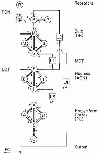Figure 4.1 Lumped circuit diagram of the sets of neurons in the olfactory bulb (OB), the anterior olfactory nucleus (AON), and the prepyriform cortex (PC). PON, primary olfactory nerve; LOT, lateral olfactory tract; EC, external capsule; R, receptors of the nasal mucosa; gl, glomeruli; P, periglomerular neuron; M, mitral neuron; G, granule cell; E, superficial pyramidal cells of AON; I, inhibitory neuron; A, superficial pyramidal neuron; B, short local interneuron; C, deep pyramidal neuron; +, excitation; −, inhibition; L, latency. (Adapted from Freeman WJ. Analytic techniques used in the search for the physiological basis of the EEG. In: Gevins A, Remond A, eds. Handbook of Electroencephalography and Clinical Neurophysiology, vol. 1: Methods of Analysis of Brain Electrical and Magnetic Signals. Amsterdam: Elsevier; 1986.)

With these general objectives in mind, this chapter considers a few models of the generation of EEG phenomena that have been elaborated in the past decades. We focus here on models of EEG rhythmic activities both at the macroscopic and the microscopic level. The former are simplified models in which detailed mechanisms are kept to a minimum and the main properties of subpopulations of neurons are lumped together. These models can, however, be easily adapted to include more specific neuronal properties and more complex connectivity. Taking into consideration that in this chapter we are particularly interested in dynamic models of neuronal networks that are responsible for the generation of the main properties of EEG/MEG (electro/magnetoencephalographic) signals, we pay special attention to macroscopic models. It should be emphasized that the brain is a very complex system, and even one cortical column consists of a large number of elements, neurons, ionic channels, synapses, neurotransmitter systems, and glial cells that require enormous amount of parameters and state variables for a proper description. The dynamics of EEG/MEG signals, however, can be accounted for within the framework of systems operating within spaces with much lower dimensions. This is the realm of macroscopic models, namely neural mass models (NMMs) that use mean field concepts, where the properties of subpopulations of neurons are lumped together based on the fact that many neurons within a given neuronal system share basic properties. Nonetheless we also consider, albeit in abbreviated form, some results of studies using microscopic models that are also relevant for understanding some characteristics of EEG/MEG signals. In this respect the models developed by Edelman and collaborators (4) are good examples of models that combine detailed properties of neurons and synapses within large-scale systems. Although these models have been introduced mainly to study functional connectivity at different scales of complexity with respect to neurocognitive processes, their capacity to generate brain rhythms and EEG-like phenomena should also be stressed. It is to be expected that the applications of this new generation of large-scale computer models of complex neuronal networks will grow fast in the coming years, since these kinds of models can now be realized by virtue of the current availability of powerful computer systems. An ambitious project along this research line is the Blue Brain project that has the aim of creating a synthetic mammalian brain by reverse-engineering, using IBM’s Blue Gene supercomputer, in order to investigate the brain’s architectural and functional principles underlying cognitive processes (5).

Another new trend is the development of Topological Models of neuronal networks with their patterns of connectivity that can be studied using the mathematical theoretical approach of “small-world” graphs. These are mathematical graphs that consist of nodes that can be reached from every other by a small number of steps, which have been applied in a wide variety of fields, from gene to social networks. Watts and Strogatz (6) classified such graphs according to two independent structural features, namely the clustering coefficient and average node-tonode path length. This approach is in essence an analytical tool that can extract interesting parameters to characterize functional connectivity within networks of cortical neurons and conditions determining neuronal synchrony (7,177) and to analyze fMRI and MEG/EEG data (8), but it has not addressed explicitly the question of the generation of EEG/MEG activities.

MACROSCOPIC MODELS OF EEG GENERATION

Basic Principles: The Wilson-Cowan Approach

At the macroscopic level we describe NMMs that are based on the mean-field approximation approach. Under this heading we consider two classes of models: (i) models that account for
time-dependent properties of neural populations and (ii) models that include, in addition, space-dependent properties. In general terms this approach was introduced in a systematic way in the Neurosciences by Wilson and Cowan (9) who proposed a theoretical framework that emphasizes not the properties of individual cells but rather those of neuronal populations. A basic assumption is that cortical neurons form a dense network consisting of, at least, two subpopulations that are interconnected either directly or by way of interneurons. The basic variable is the proportion of neurons of each subpopulation that are active at a given time, such that the relevant variable is not the single spike but the average spike frequency. The dynamics of the neural mass depends on the interaction of excitatory and inhibitory neuronal subpopulations. Accordingly the model requires the use of two variables E(t) and I(t), describing the activity of the excitatory and inhibitory subpopulations, respectively, to characterize the state of the whole population.

Based on these assumptions the general Wilson and Cowan equations (9) governing the dynamics of a localized population of neurons were derived:

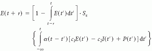
and

This formalism describes the activities of the excitatory E(t) and inhibitory I(t) subpopulations; c₁ and c₂, and c₃ and c₄, are the connectivity constants representing the average number of excitatory and inhibitory synapses per cell for each subpopulation, α is the decay time constant, S_e(x) and S_i(x) are the response functions that give the expected proportion of cells in a subpopulation that would respond to a given level of excitation and are represented by sigmoid functions; P(t) and Q(t) are the external inputs to the excitatory and the inhibitory subpopulations, respectively; r is the refractory period.

Neural Mass Models of EEG Rhythms

Based on the theoretical formalism introduced by Wilson and Cowan (9), Lopes da Silva et al. (10) described an NMM with the aim of simulating the conditions under which alpha rhythms occur. The model consisted of lumped subpopulations of interconnected excitatory and inhibitory neurons with properties of thalamocortical cells and a special subpopulation of interneurons. The mathematical analysis was initially carried out for a linearized approximation of the neuronal network in order to express the transfer function of the network and the power spectrum of the average membrane potential. The latter was interpreted as the local EEG signal, which in this case consisted of a predominant alpha rhythm. Later the analysis was extended to take into account a first approximation of the nonlinear behavior (11). In the section of alpha rhythms we describe these models in more detail.

More recently these kinds of models were extended to account for EEG frequency components other than the alpha rhythms.

In this context the model study of Jansen and Rit (12) marks an important advance. These authors introduced a lumped-parameter model of a cortical column consisting of a population of pyramidal cells interconnected with populations of excitatory and inhibitory interneurons, which displays five kinds of simulated EEG outputs when fed with random noise. These different EEG outputs are the following: low amplitude noise for high values of the inhibitory feedback, slow periodic activity similar to that obtained in comatose patients, typical alpha rhythmic activity, noisy alpha activity, and low-amplitude high-frequency activity similar to beta activity for high values of the excitatory feedback. In order to explore how different cortical columns interact, Jansen and Rit investigated the behavior of two identical single-column models and showed that they may produce in-phase oscillations.

Another case where NMMs of interacting neuronal populations helped to clarify the origin of a specific EEG/MEG phenomenon was studied by Suffczynski et al. (13). This phenomenon is the so-called focal ERD-surround ERS, described in detail in Chapter 45, where a given event (e.g., finger movement) can cause at the same time a decrease (event-related desynchronization or ERD) and an increase (event-related synchronization or ERS) of EEG/MEG power within the alpha frequency range (mu rhythm) depending on the site over the scalp. The analysis of coupled NMMs representing thalamocortical systems responsible for the hand and for the foot movements, respectively, was able to reveal how this reciprocal “ERD-ERS” phenomenon takes place.

Based on the results obtained with NMMs generating rhythmic activities within the alpha frequency range, several researchers extended these models to account for different EEG frequency bands besides the alpha rhythm. In this respect, David and Friston (14) described a lumped model that generates various rhythmic activities ranging from delta to gamma, according to the kinetics of the populations included in the model. These authors also investigated the dynamics of the interaction between different cortical areas by coupling two lumped models. Depending on coupling strength, direction of coupling (unidirectional or reciprocal coupling), and propagation delays, they showed that the oscillation frequency depends on the delay and that a reciprocal coupling is characterized by oscillatory signals in phase or in antiphase. This latter result reproduces the experimental finding of zero-lag synchronization among remote cortical areas as found experimentally by Roelfsema et al. (15) and Chawla et al. (16).

With the aim of investigating how different cortical regions can display complex EEG frequency spectra and several patterns of functional connectivity, Zavaglia et al. (17,18) also developed interconnected lumped models. They showed that three populations, consisting of four subpopulations (pyramidal neurons, excitatory, slow, and fast inhibitory interneurons), arranged in parallel are sufficient to account for complex EEG
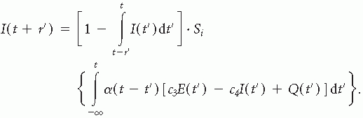
spectra with dominant frequency ranging form theta to alpha and gamma. This model is akin to the comprehensive NMM introduced by Wendling et al. (19) to account for the generation of different kinds of neural activities and the corresponding EEG signals, including epileptic activity as described in more detail in the section dedicated to models of epileptic phenomena generated by neural populations. This model illustrates very clearly the main features of the currently used NMMs (Fig. 4.2).

Figure 4.2 (a): Neural mass model consisting of a subpopulation of principal cells (pyramidal cells) that project to and receive feedback from subpopulations of local interneurons. Feedback to pyramidal cells is either excitatory (recurrent excitation) or inhibitory: dendritic-projecting interneurons with slow synaptic kinetics—IPSP (slow)—shown in (c)—and somatic-projecting interneurons (gray hexagon) with faster synaptic kinetics—IPSP (fast)—shown in (c). (b): Corresponding block diagram representing for each subpopulation, the average pulse density of afferent action potentials that is transformed into an average inhibitory or excitatory postsynaptic membrane potential using a linear dynamic transfer function with impulse response h_EXC(t), h_SDI(t), and h_FSI(t) while this potential is converted into an average pulse density of action potentials fired by the neurons by way of a static nonlinear function (asymmetric sigmoid curve, S(v)). Interactions between main cells and interneurons are represented by seven connectivity constants (C₁ to C₇), which account for the average number of synaptic contacts. One of the model outputs represents the summated average postsynaptic potentials on pyramidal cells. It simulates an EEG signal. The three main parameters of the model respectively correspond to the average excitatory synaptic gain (EXC), to the average slow inhibitory synaptic gain (SDI), and to the average fast inhibitory synaptic gain (FSI). (Adapted from Wendling F, Hernandez A, Bellanger JJ, et al. Interictal to ictal transition in human temporal lobe epilepsy: insights from a computational model of intracerebral EEG. J Clin Neurophysiol. 2005;22(5):343-356.)

Neural Mass Models with Spatial-Temporal Features—Continuous Neural Field Models

In addition to the lumped NMMs described above, where spatial aspects are not explicitly simulated, there are also models that include spatial properties and consist of spatiotemporal chains of different subpopulations of neurons. An example is the model of van Rotterdam et al. (20) that consists of a series of pyramidal cells and interneurons interconnected by means of recurrent collaterals
and inhibitory fibers with connectivity functions assumed to be homogenous while the strength of the connectivity was an exponentially decreasing function of distance. This model was constructed to study the factors that determine the propagation of alpha waves along a cortical sheet. Assuming a continuous chain of neurons the model’s output, u(x,t), is the space-averaged membrane potential density of the main cells. To study propagation properties in the neuronal chain an expression has been derived as a linear inhomogenous partial differential equation by means of which one can determine group velocity of alpha waves and dispersion properties. Alternatively the neuronal chain may be conceived as a two-dimensional system with a specific transfer function relating a random input p(x,t) to the output u(x,t). The model results were able to emulate experimental data, namely the propagation velocity that was found experimentally in the canine cortex to be about 0.3 m/sec (21) based on parameters taken from physiology and histology, as explained further in more detail in this chapter.

A series of other models, akin to that of van Rotterdam et al. (20), where the cortical neuronal populations are modeled as forming a continuum have been made, including models incorporating stochastic features called continuous neural field models. In this chapter we focus on those aspects that are specifically relevant for EEG/MEG generation, while the more general aspects of cortical processing of information with respect to neurocognitive functions lie outside the scope of this text. With respect to these continuous neural field models, in general, the reader may be referred to comprehensive reviews of Harrison et al. (22), Deco et al. (23), and Jirsa (24). Examples of continuous neural field models are those of Jirsa (24,25) and of the Australian group (26, 27, 28 and 29). Jirsa (24) gives a very thorough account of how a set of state equations with parameter values based on physiology can account for the dynamics of cortical neuronal populations at different spatial scales: microscopic, mesoscopic, and macroscopic. At microscopic level, fast synaptic feedbacks appear to be crucial to the stability of the excited cortex. At mesoscopic scale the model shows how fields of synchrony can be established, and at macroscopic scale it shows how traveling waves may be generated in the cortex. The last two levels are particularly relevant with respect to the dynamics of EEG/MEG generation. With respect to these models the activity state of a single neuron can be described by its membrane potential, V, the capacitive current, I, or the time since the last action potential, T. Each of these variables can be represented by a dimension in the phase space of the neuron’s activity state. Accordingly this phase space would be three-dimensional and the state of a neuron would correspond to a point v = {V,I,T} or particle in phase space. Using a general formalism the activity state of a population of neurons at any time, t, can be described in phase space by a density p(v,t). As the state of each neuron evolves the ensemble density, p(v,t) evolves until it reaches some steady state. The evolution of the ensemble density dynamics can be described using the formalism of the Fokker-Planck equation. The latter describes in general terms the time evolution of the probability density function of the position of a particle in a given multidimensional space. The interested reader may find a thorough treatment of the applications of this formalism in the study of continuous field models by Deco et al. (23) and Harrison et al. (22).

Neural Mass Models and Hemodynamic Signals

NMMs are also being applied to make a bridge between the activity of neuronal networks as reflected in EEG signals and hemodynamic signals as measured by way of functional MRI, in order to understand better the working of cortical networks underlying cognitive processes. This constitutes a central feature of dynamic causal modeling (DCM) (30) that has been applied not only to fMRI signals but also to electrophysiological signals such as event-related potentials (ERPs) (31).

Valdés-Sosa et al. (32) proposed an approach where the summed postsynaptic potentials generated by an NMM of a cortical area are used in the forward mode to estimate the primary current density distribution of a cortical area (Fig. 4.3). This is then transformed into the signal recorded at EEG sensors by applying a linear spatial convolution with the EEG lead field, that is, the function that relates any source in the brain to the corresponding measurements at the EEG sensors. Simultaneously the summed postsynaptic potentials generated by the NMM are transformed into a local Vasomotor feed forward signal that is then further transformed by way of a temporal convolution with the hemodynamic response function (HRF) into a simulated BOLD signal. In this way the information obtained from the EEG signal and from the corresponding fMRI BOLD signal recorded from the same region of interest can be fused (Fig. 4.3). We should note that although this approach opens interesting novel perspectives and
merits being further elaborated, it is based on concepts that are still insufficiently established. Namely more research is needed to better understand how neural activities, generated by neural populations with complex geometrical configurations, are transformed into cortical current distributions on the one hand, and how they are associated with BOLD signals on the other.

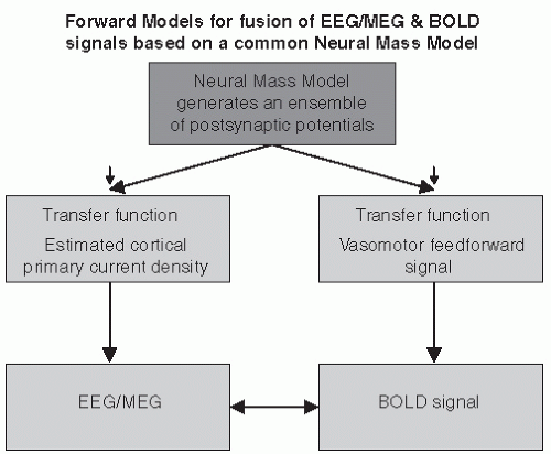Figure 4.3 The output of a neural mass model in the form of summed postsynaptic potentials can be used to estimate the primary current density distribution of a cortical area that is transformed into the EEG/MEG signal. Simultaneously the summed postsynaptic potentials generated are transformed into a local Vasomotor feed-forward signal that is then further transformed by way of a temporal convolution with the hemodynamic response function into a simulated BOLD signal. In this way EEG/MEG information can be fused with the corresponding fMRI BOLD signal recorded from the same region of interest. (Inspired from Valdes-Sosa PA, Sanchez-Bornot JM, Sotero RC, et al. Model driven EEG/fMRI fusion of brain oscillations. Hum Brain Mapp. 2009;30(9):2701-2721.)

MODELS OF SPECIFIC EEG ACTIVITIES

Here we describe a number of models that account for the generation of specific types of EEG activities, namely the following:

Models describing the generation of the EEG of olfactory areas of the brain as proposed extensively by Freeman (1) and later further elaborated (33,34) that may be considered paradigmatic of neural mass modeling approaches;
Models of alpha rhythms of the thalamus and cortex, since these are one of the most conspicuous features of the human EEG, as proposed by Lopes da Silva et al. (10,11) and elaborated in more detail by van Rotterdam et al. (20), and extended later by Jansen and Rit (12), Nunez (35), Wright and Liley (36), Stam et al. (37), Valdes et al. (38), Robinson et al. (39), Suffczynski et al. (13), David and Friston (14), and Zavaglia et al. (17,18);
Detailed models of membrane and synaptic properties of thalamic cells and circuits responsible for the generation of 7- to 14-Hz spindle rhythmicity that occurs at the onset and in the light stages of sleep, based on the experimental findings of Steriade et al. (40, 41, 42, 43, 44, 45, 46, 47 and 48);
Models of epileptiform EEG, namely of absence seizures, that display complex nonlinear dynamics, namely bistable behavior, where abrupt transitions occur between two states—normal and paroxysmal (49,50)—and of epileptic seizures of the limbic cortex (19,51), as well as detailed models of the generation of epileptiform transients by Traub (52), Traub and Wong (53), Traub et al. (54,55), and Traub and Miles (56);
Models of beta and gamma rhythms developed by Traub et al. (57) with realistic simulations of synapses (55,57, 58, 59 and 60). We do not include here models of hippocampal theta rhythms since the basic physiology of these rhythmic activities has already been described in Chapter 3.

Model of Olfactory Area EEG

The main neuronal populations of the olfactory brain structures that are of importance for an understanding of the generation of the olfactory EEG can be summarized as follows: in the bulb, the mitral and tufted cell (M) population, which is excitatory, and the granule cell (G) population, which is inhibitory; in the PC, the surface pyramidal population, which is excitatory (E), and the basket cell population, which is inhibitory (I). The interaction between the M and the granule neuron populations forms an inhibitory feedback loop. The interaction between the surface pyramidal and the basket cell populations in the PC also forms an inhibitory feedback loop (Fig. 4.1).

As can be seen in Figure 4.1, there are also mutual excitatory interactions between M neurons in the bulb and between pyramidal A neurons in the PC, as well as mutual inhibitory interactions between granule cells in the bulb and basket cells in the prepyriform cortex (PC). Excitation of the M cells by primary olfactory nerve (PON) inputs leads to excitation of the granule (G) neurons and to feedback inhibition of the M neurons. In consequence, the G neurons are disexcited and the M neurons are disinhibited. In this way, the M neurons may become excited again, and the whole process may continue in an oscillatory mode. The basic oscillation is at 40 Hz in cat and 60 to 80 Hz in rabbit (61). A similar type of inhibitory feedback loop occurs in the PC, and the EEG of this cortical structure resembles that of the olfactory bulb (OB) in frequency content. In this model and similar ones, the action potentials are converted into graded currents at the somadendritic synapses causing the postsynaptic potentials. In a first approximation, these postsynaptic potentials may be considered to sum at the soma. At the trigger zone, the axon hillock, these potentials are transformed into spike trains depending on a threshold.

The postsynaptic potentials may be considered as the wave (W) mode of operation of the neural set; the action potentials represent the pulse (P) mode. This is, of course, a simplification of processes taking place at the membrane, but at the level of generalization at which NMMs of the EEG are constructed, these are the main features that must be considered. The sensitivity of the threshold process in the bulb and cortex is controlled by centrifugal influences that originate in the forebrain and brainstem, among others from the locus coeruleus (62). The conversion between the postsynaptic potential (W mode) and the pulse rate (P mode) may be given in terms of the sigmoid curves shown in Figure 4.4 for a single neuron and for the population or ensemble. The wave-pulse conversion can be considered as a static sigmoidal nonlinearity at the single neuron level. However, over small signal ranges this relation may be assumed to be linearized, and therefore it may be represented by a simple coefficient. To simulate the local dynamics of the EEG, delays due to synaptic and conduction processes may be accounted for by a stage of integration. Along these lines, the dynamics of these structures may be represented by a mathematical model consisting of coupled differential equations that incorporate static nonlinear functions (for a mathematical treatment see Refs. 1, 34, and 63). The main input to the populations of the OB comes from the olfactory mucosa and is modulated by the respiration rate. A study of the behavior of the KII set described above shows that this set has multiple stable states. Two are of particular interest because they represent the most common situations. The first is a quasiequilibrium state that is maintained by a steady input of low intensity; the second is the so-called carrier state (34), characterized by a limit cycle with quasisinusoidal EEG activity at 40 Hz (cat) or 60 to 80 Hz (rabbit) that occurs during inspiration. This nonlinear oscillation represents a limit cycle because the feedback gain is displaced to the excitatory side of the resting value with an increase in pulse input (either of sensory origin or depending on arousal level) that may drive the KII set out of the equilibrium state. Certain drugs such as carbachol or picrotoxin can induce a limit cycle state of long duration (34). A later section shall consider the relevance of nonlinear dynamics such as the theory of deterministic chaos for understanding EEG generation. Here it is sufficient to observe that the EEG signals simulated by the set of nonlinear coupled differential equations that describe the KII set approximate the experimentally recorded EEGs.

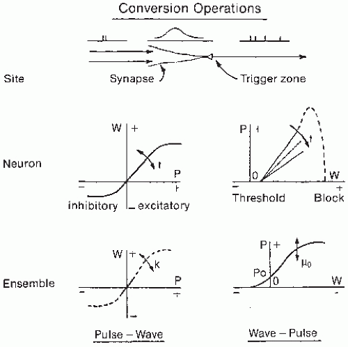Figure 4.4 Conversion operations between the wave mode (W) and the pulse mode (P) for a neuron and an ensemble of neurons. At the neuronal level both operations are time-varying (t); the P-W conversion is nonlinear; the W-P conversion is linear between threshold and cathodal block. At the ensemble level, the P-W conversion is restricted to a small linear range and W-P conversion is static and nonlinear. The derivative of this curve defines the gain; this may change (µ_o) depending on arousal level. The P-W conversion can vary to represent synaptic changes occurring with learning. (Adapted from Freeman WJ. Dynamics of image formation by nerve cell assemblies. In: Basar E, Flohr H, Haken H, et al., eds. Synergetics of the Brain. Berlin: Springer-Verlag; 1983:102-121.)

Alpha Rhythm Models: Spatial and Temporal Characteristics

A current view in neurophysiology is that the origin of certain rhythmic electrical activity seen in the EEG, such as that characteristic of some thalamic nuclei and cortical areas after administration of a barbiturate (64,65) and possibly also that occurring spontaneously, such as sleep spindles and alpha rhythms (66,67) is to be found in populations of neurons characterized by the interaction between excitatory and inhibitory neuronal populations. Different types of models have been developed to account for the generation of EEG rhythmic activities within the alpha frequency range. Some of these models operate at the microscopic level of the single neuron or the small local network (68,69), others at the macroscopic level with the aim of accounting for global properties of EEG signals recorded from the scalp (not limited to alpha rhythms) (35). Recently attempts have been made to combine the local and the global levels within a synthetic theoretical framework, among others by Nunez who developed a thoughtful “marriage of local and global theories” (Chapter 11 in Ref. 35). A particular interesting discussion of this issue is the paper of Wright and Liley (36) followed by a wide-open peer commentary.

At the cellular level, an important issue that has been repeatedly discussed in studies of the mechanisms underlying EEG rhythmic activities is the question of whether such rhythms are caused by single cells with pacemaker properties. A significant advance in this discussion was achieved when it was demonstrated by Jahnsen and Llinás (70,71) that some types of thalamic neurons display oscillatory behavior in vitro, even after blockage of synaptic transmission. Most neurons studied in this way tend to generate oscillations in the frequency range of 6 to 10 Hz. These intrinsic oscillatory properties of some neurons are most likely of importance in shaping the rhythmic behavior of the networks to which they belong. However, these properties may not be sufficient to account for the network rhythmic behavior. One main argument supports this statement: the disconnection of cortically projecting thalamic cells from their inputs, which arise in the reticular (RE) nucleus of the thalamus, abolishes spindles in thalamocortical relay (TCR) neurons (72). However, single TCR neurons may preserve their intrinsic membrane oscillatory properties in vitro (70,71). Interestingly, the capacity of both TCR-RE circuits and the isolated RE nucleus, in vivo, to generate spindle oscillations contrasts with the fact that the RE nucleus isolated in vitro does not show spontaneous oscillations (73, 74, 75, 76, 77 and 78). This is likely because the input conditions of the RE neurons in vitro are different from the situation in vivo because the neurons lack neuromodulation influences, including cholinergic, noradrenergic, and serotoninergic inputs. In modeling studies, the influence of neuromodulators on RE neurons membrane potential was simulated (68), namely noradrenaline and serotonin, by blocking leak K⁺ currents and thus depolarizing the RE neurons to the same level as observed in vivo. These studies showed that waxing-waning oscillations could occur in the RE network, similar to those seen in vivo. This finding provides clear evidence that the oscillatory behavior of these neuronal populations of RE neurons depends on specific levels of the neuronal membrane potential that is affected by several inputs, both at short- and long-range. Among the latter, the neuromodulatory inputs arising from the raphe nucleus (serotoninergic), the locus coeruleus (noradrenergic), as well as glutamatergic projections form forebrain areas are particularly important. Among the former it is interesting to note that gap junctions have been shown to exist between RE nucleus (79) and thus may also participate in the modulation of their oscillatory properties.

To understand how oscillations may be generated in thalamic nuclei, we must consider the basic structure of these neuronal networks. In the thalamic relay nuclei where this type of rhythmic activity can be recorded, namely the relay nuclei of the thalamus, three main types of neurons can be distinguished (see also Chapter 3 for a discussion of the physiology of these cellular elements): the TCR neurons, whose axons project to the cortex; the RE nucleus neurons that contribute to the inhibitory feedback control of the former; and the local, intrinsic, neurons. The RE forms a thin sheet of neurons that surround the anterior and lateral side of the thalamus and interact synaptically with the TCR neurons. The axons of the RE cells have as main target the TCR cells. Their dendrites make synaptic contacts with the axons of the TCR cells. Thus the TCR and the RE neurons are interconnected by means of a feedback loop as schematically shown in Figure 4.5. Both the RE and the local-circuit neurons contain aminobutyric acid (GABA) as transmitter. This implies that the feedback of the RE on the TCR
neurons is GABAergic and thus inhibitory. The RE neurons receive fast GABA_A-mediated inhibitory postsynaptic potentials (IPSPs) from neighboring RE neurons; in this way these neurons form a chain of cells interconnected by inhibitory synapses. In addition they receive fast glutamatergic (AMPA type) excitatory postsynaptic potential (EPSPs) from TCR neurons. In turn the TCR neurons receive both fast GABA_A and slow GABA_B IPSPs from RE neurons (74,75). In a thalamic nucleus, a number of feedback circuits between TCR and RE neurons can be distinguished.

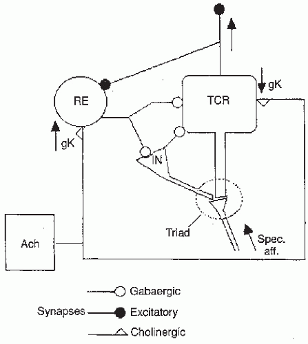Figure 4.5 Simplified scheme of a thalamic neural network where the main features are presented. The thalamocortical relay (TCR), the reticular thalamic (RE), and the local-circuit interneurons (IN) are indicated, along with projections from a cholinergic population (ACh). The synaptic triad formed by the dendrites of TCR and IN neurons with the specific afferent (spec. aff.) fibers is also indicated. Three types of synapse are shown: excitatory, aminobutyric acid (GABA)ergic (inhibitory), and cholinergic. The effect of the latter on RE neurons is assumed to be an increase in potassium conductance (g_k), whereas on the TCR neurons the effect is the opposite. (From Lopes da Silva FH. Neural mechanisms underlying brain waves: from neural membranes to networks. Electroencephalogr Clin Neurophysiol. 1991;79:81-93, with permission.)

In the context of this discussion, it is important to note that the TCR neurons can work essentially according to two distinct modes: either (a) as relay cells that simply depolarize and can produce single spikes in response to an adequate input volley or (b) as oscillatory cells producing bursts of high-frequency spikes that are repeated in a rhythmic fashion. The resting membrane potential of a TCR neuron determines whether such a neuron will be active in the relay or in the oscillatory mode. To understand this question, it is necessary to take into account the intrinsic membrane properties of these cells, namely their main ionic conductances and the corresponding dynamics. It should be noted that these properties became known mainly due to microphysiological investigations in thalamic slices, in vitro, and in isolated brain preparations by the groups of Llinás and collaborators (70,71). For a comprehensive account of these membrane properties, the reader is referred to the original publications and to the excellent reviews by Steriade and Llinás (80), Steriade et al. (66,67), McCormick (81), McCormick and Bal (82), Destexhe et al. (69), Destexhe and Sejnowski (83), (84), Lörincz et al. (85), and to Chapter 3.

A basic question is whether the different types of oscillations can be found in vitro in the absence of external inputs, since this would give support to the idea that these thalamic cells may support pacemaker rhythmic activity. Jahnsen and Llinás (70) provided an initial answer to this question by showing that the oscillatory activity at about 10 Hz may be observed in the absence of external drive in vitro. However, we must also consider what is the contribution of the feedback circuits between TCR and RE neurons to the generation of EEG oscillations in vivo.

In this context the most direct experimental evidence pertains to the generation of spindle oscillations occurring during the early stages of sleep. Spindles appear in the EEG of most mammals as oscillations with a frequency in the range from 7 to 14 Hz, which form bursts lasting for 1.5 to 2 sec that recur periodically with an irregular periodicity of about 5 to 10 sec. This type of spindle can also be seen in animals under barbiturate anesthesia. It was shown by Steriade et al. (72) that no thalamic nucleus is capable of generating spindle oscillations after disconnection from the RE nucleus. Therefore, the existence of feedback circuits including the RE nucleus is necessary for spindling to occur under normal conditions in vivo. Nonetheless there are other mechanisms that may be responsible for alpha rhythmic generation at least in brain slices in vitro but have not been incorporated in explicit models as described by Lörincz et al. (85) and in Chapter 3.

In conclusion, under the normal conditions of an intact brain, both synaptic interactions and input signals play an essential role in setting the conditions necessary for oscillatory behavior to occur. The frequency of this oscillation depends on the intrinsic membrane properties on the membrane potential of the individual neurons and on the strength of the synaptic interactions.

Simplified Distributed Network Model

A simplified model has been proposed (10,11) that incorporates the limited physiological and histological data available at that time; these assumptions were sufficient to explain the generation of the alpha rhythm, that is, the EEG stochastic signal that lies in the frequency range of 8 to 13 Hz. This appears mainly at eye closure and can be recorded best from the posterior regions of the scalp in humans. A similar type of activity has also been recorded at the visual cortex and some thalamic nuclei in dogs (86) and cats (87,88). The model in its most simple form consists of a set of simulated neurons, thalamocortical relay (TCR) cells, and interneurons (INs). The latter may be assumed to be the RE cells as shown in Figure 4.5, although the IN cells shown in this figure may have a complementary effect. For simplicity in the model, the cells providing feedback are denoted, in the following, as INs. In contrast with the lumped
models, some examples of which have been given for the olfactory system, this model is a distributed one in the sense that each neuron is modeled individually; it occupies a specific position within a matrix of neurons. Such a distributed model offers some special possibilities for theoretical studies that are not easily available in lumped models.

Without entering into great detail about the alpha rhythm distributed model, it is of interest to point out some of its characteristics. First, the structure of the distributed model initially used (10) consisted of 144 TCR neurons and 36 INs; the 32 TCR neurons that surrounded one IN were responsible for its excitation, while each IN was responsible for the inhibition of the 12 TCRs around it. The excitation and inhibition were represented by time functions that were an approximation of the waveforms of EPSPs and IPSPs, respectively. The matrix of neurons should be viewed as lying at the surface of a torus. Furthermore, each neuron fired whenever the membrane potential exceeded a simple threshold; a short refractory period then followed. A basic characteristic of this model was that the input received by each TCR neuron was in the form of a series of pulses (action potentials) that had a Poisson distribution; the inputs to the individual TCR neurons were uncorrelated. The model’s output signal was the sum of the membrane potential fluctuations of all TCR neurons. This output signal simulated the general spectral properties of an alpha rhythm. This result is illustrated in Figures 4.6, 4.7 and 4.8.

Only gold members can continue reading. Log In or Register to continue