Fig. 2.1
Chromosomal organization
The DNA contained in the chromosomes provides the blueprint for making all the structures inside the human body, as well as all the “software” needed to regulate its processes at the molecular level. All the necessary information is stored in the DNA sequence as a series of codes. A sequence of DNA that contains coding information is called “exons,” while non-coding sequences are called “introns.” A series of steps occur inside each cell to decode these information and translate them into protein products that are essential for metabolism as well as other normal functions of the human body. Through the process of transcription, a single DNA strand is used as a template for constructing a complementary RNA strand. Apart from the intrinsic chemical difference between DNA and RNA, the most important difference is that U (uracil) replaces T in RNA. In a certain region of the genome, which we call a gene, the transcribed RNA sequence encodes for information (codons – every three bases of RNA determine an amino acid) on how to make a certain protein (depending on the gene) with a specific amino acid sequence. Any genes will contain regulatory sequences and variable numbers of intervening exons and introns. The transcription of genes forms messenger RNA (mRNA) and would include all the intron and exon regions. Although the introns are non-coding region and are removed eventually, they may have regulatory functions during the processes of transcription. Eventually with post-transcriptional modification called splicing, these intron regions are removed, and the coding exons are linked together to form mature mRNA. The mRNA then undergoes translation. This is the process in which the specific amino acid sequence coded for by the mRNA is translated by ribosomes into amino acids. The amino acid sequences assemble into peptides and proteins (Fig. 2.2). Upon further post-translational folding, twisting, and interacting with other proteins, the secondary, tertiary, and quaternary structure of proteins are formed. These are important for the proper functioning of the active protein.
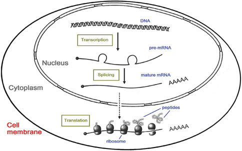
Fig. 2.2
Central dogma from DNA through RNA to protein
These proteins may form part of the structural elements of the tissue, such as collagen types 1 and 2; they may contribute to the extracellular matrix to form proteoglycans; or they may form regulatory enzymes, such as metalloproteinases, that help to regulate the metabolic processes inside the tissue.
2.1.2 Genetic Polymorphisms and Their Relation to Diseases
The haploid genome is comprised of about three billion base pairs (bp). There are about 30,000 genes located in the genome [40, 81]. Majority of the genome is shared in common among the population, with only a small part of it having variation. Such small proportion of difference may cause great influence on the phenotype of different individuals. The two most common types of variation, also called polymorphisms, are microsatellites and single nucleotide polymorphisms (SNPs). At the locus where the polymorphism is located, variants are called alleles. These alleles of the polymorphism are inherited through generations with each individual having two alleles at each locus and are determined by both the paternal and maternal lineages. Microsatellites are tandem repeats of short sequence of 2–8 bp, and the number of tandem repeats differentiates alleles (Fig. 2.3). It is highly polymorphic. SNPs are polymorphisms that differ at a single nucleotide (Fig. 2.4), and the number of known SNPs exceeded ten million in the human genome [15, 79]. Although an individual SNP is not as polymorphic as a microsatellite due to the limited number of alleles, they are compensated for by the large numbers of SNPs scattered throughout the gene and the genome; thus with high-throughput genotyping technology, SNP markers are more commonly used for genetic analysis nowadays. There are various types of SNP, such as non-synonymous coding SNPs that change the amino acid sequence encoded, synonymous coding SNPs that do not modify the encoded amino acid, intronic SNPs located in the introns that might affect proper splicing, SNPs located in the 5ʹ and 3ʹ untranslated region (UTR), and intergenic SNPs that are not located within a gene.
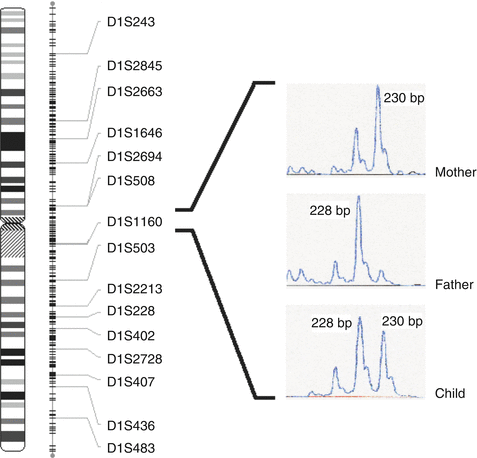
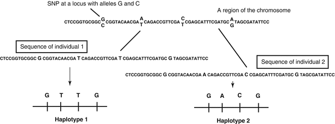
Fig. 2.3
Microsatellite markers and their inheritance. The mother is homozygous for 230 bp allele at marker D1S1160, while the father is homozygous for 228 bp allele. As a result, their child inherited one copy of both alleles simultaneously from the parents and hence heterozygous at the marker
Fig. 2.4
SNP and haplotype. On the sequence of a chromosome region, there are four SNP loci. When considering the haplotype of these four loci, individual 1 is having GTTG, while individual 2 is having GACG
Changes in gene sequences that result in disease are generally called mutations, while changes in the gene sequence without significant external effects are termed polymorphisms. Nonsense mutations result in an amino acid change to a stop codon. Deletion mutations delete one or more nucleotides from a sequence, and insertion mutations insert one or more nucleotides into a sequence. The most recorded pathogenic mutations are detected in the coding sequence such as nonsynonymous mutations and frameshift mutations. Promoter is the regulatory region that is located upstream of a gene, and it provides regulation to transcription so that gene expression is controlled. Mutations in promoter which controls gene transcription would prevent the promoter from working, resulting in a change in the level of gene expression. These products of mutations may have reduced or no function, called loss of function mutation [7], while gain of function mutation takes place when the gene product has a positively abnormal effect [30, 68].
If we are referring to a single locus, the term genotype is used to define the status of the two alleles. On the other hand, when more than one locus on a chromosome is considered, haplotype denotes their allele configuration according to their order in physical position (see Fig. 2.4). Since a single SNP locus has only two alleles, it is not very polymorphic, with a limited number of variations. Thus several SNP loci can be combined into a haplotype and used to increase the power to detect associations (see Fig. 2.4).
With the advance of sequencing technologies [5, 35], sequencing of individual human genomes or whole exons (1–2 % of the human genome) is becoming more and more affordable. The technologies allow discovering every type of DNA variations in genome, not just most common variations (SNPs and microsatellites) we mentioned above but also other variations such as rare alleles (low-frequency alleles), copy number variations (CNVs). These variations may explain some more genetics effects for disease phenotypes and can be used as markers to study the relationship between genotypes and phenotypes.
2.1.3 Types of Disease
Phenotypic variations between individuals are determined by polymorphisms of particular genes resulting in differences in genotypes. These phenotypic outcomes may be expressed subtly at the molecular level (e.g., expressional level difference of a protein) or more obviously resulting in notable body changes (e.g., height) or even symptoms of diseases. However, risk-conferring genotype in one individual may not necessarily result in disease or symptoms of disease in another. This is because of a phenomenon known as penetrance. Incomplete penetrance refers to the case in which the risk-conferring genotype is not fully expressed and therefore does not actually cause disease. This maybe because the risk-conferring genotypes may require additional exposure to environmental factors, as well as interaction with other susceptibility genes in order to develop disease. Such conditions requiring an interaction of multiple genes with the environment are known as complex genetic disorders. Osteoarthritis, degenerative disc disease, hypertension, and diabetes are examples. Mendelian disease refers to a simpler form of disease in which alternation or mutation at a single gene is enough for its manifestation [56, 61]. They represent rare diseases with more severe phenotype, such as osteogenesis imperfecta or Duchenne muscular dystrophy. Furthermore, phenotypic outcomes may be qualitative (i.e., with or without the disease) or quantitative, presenting with a spectrum of severity from mild to severe, which can be measured by number of units (e.g., blood pressure, scores of intervertebral disc degeneration) [72].
2.2 Disease Gene Mapping
Before claiming that a disease has a genetic component and trying to find the gene, commonly called mapping, it is important to estimate the relative importance of the genetic risk factor on the disease. One way to do so is to assess familial aggregation; if the disease occurs in multiple members of the same family, this is an indication. However, one needs to remember that members of the same family are likely to be exposed to similar environmental factors, such that the appearance pattern of a disease may not be ultimately due to genes but merely to non-genetic factors. On the one hand, an even better method is to examine disease occurrence between twins, especially as monozygotic (identical) twins share the same genes; on the other hand, dizygotic (non-identical) twins only share 50 % of similar genes. Therefore, for a purely genetic disease, the monozygotic twins should both have the disease (high concordance rate). But if both monozygotic and dizygotic twins have similar concordance rates, it would be stronger evidence for shared environmental factors being a major factor. If low concordance rates are found among twins, the disease could be affected by some unshared environmental factors. In summary, for a disease predisposition to be genetic, high and low concordance rates must be obtained from monozygotic and dizygotic twin pairs, respectively [9]. These classical twin studies are a common feature of many diseases that are suspected to have a genetic component.
Once a disease has been confirmed to have a substantial genetic component, one can attempt to map the disease gene to a particular location in the genome by the use of a number of strategies including linkage analysis on familial subjects, case-control association studies using population-based subjects on either biologically relevant candidate genes, or case-control association studies on a genome-wide scale using gene-chip arrays.
2.2.1 Linkage Analysis on Familial Subjects
Linkage analysis is a classical method for mapping disease genes, and it has been successfully used to identify numerous disease genes in the past decades. Families, preferably large and having multiple affected members, are recruited and genotyped for hundreds of microsatellite markers. If a disease gene is located in the proximity of one of these markers, so that recombination is unlikely to occur at a position in-between the marker and the disease gene, that region of the chromosome is likely to be transmitted to affected members within the family together with the marker. Hence, the marker is said to be in linkage with the disease gene and produces a characteristic pattern of transmission (Fig. 2.5). With the use of microsatellite markers covering the whole genome, genome-wide linkage analysis can locate the rough chromosomal localization of an unknown disease gene without any prior knowledge. It is a powerful strategy that can maximize the chance of finding a disease gene.
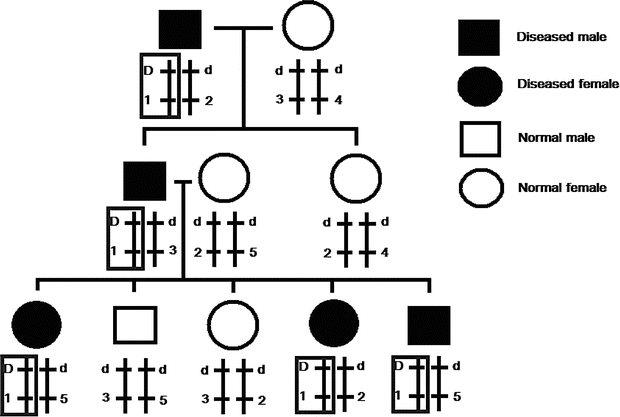
Fig. 2.5
Typical inheritance pattern of linkage. In the figure, two loci are considered. The upper locus is the disease gene locus with disease allele D and normal allele d, while the lower one is a nearby microsatellite marker locus with many alleles (1–5). If the two locus is in linkage, they will be transmitted together to the offsprings without being disrupted by recombination during meiosis. In this example, the two loci are in linkage, and allele D is linked with allele 1. The resulting haplotype D-1 is transmitted to every diseased family member. Since the disease gene locus is unknown, linkage analysis relies on correlating the marker locus inheritance (genotype) with disease status (phenotype) to detect linkage. As the marker locus is in linkage with the phenotype, it is an evidence that the unknown disease gene locus is somewhere nearby and thus its rough chromosomal localization can be determined. By using large amount of markers covering the whole genome, genome-wide linkage analysis can be performed. As the markers are not the actual disease-causing mutation and they only denote a certain status of the chromosome, each family may have a different allele in linkage with the disease-causing allele
If the marker is on the same chromosome as the disease gene, recombination will be responsible for breaking them up so that their alleles will not be transmitted together on the same chromosome. The further apart they are, the higher the chance that they will be affected by recombination. Hence, from the rate of recombination, we can estimate the distance between the marker and the unknown disease gene. Generally speaking, a 1 % recombination rate (θ) is referred to as 1 centimorgan (cM) apart, and it is roughly equivalent to one million bp distance on the chromosome [55, 69].
In a parametric linkage analysis, one tests whether the test hypothesis (that the marker is linked to the disease gene) or the null hypothesis (that the marker is not linked to the disease gene) is true. After making the assumption of disease model (e.g., mode of inheritance, penetrance, and disease allele frequency), one performs sequential test at various θ to compare the likelihoods of the test and null hypotheses. The likelihood of the test hypothesis to the likelihood of the null hypothesis is called the likelihood ratio or odds. Taking the logarithm to base 10 of this likelihood ratio will give us the LOD (logarithm of odds) score. The point with the highest LOD score indicates the most likely distance between the marker and the disease gene locus [51]. To achieve a genome-wide significant level equivalent to p = 0.05, an LOD score of 3.3 is required [39].
The advantage of the LOD score method is that one can combine the results from different studies to strengthen the significance (considering they are studying the same disease with the same disease model assumption) [51]. For instance, one may have relatively small sample sizes across studies and find suggestive linkage evidence with LOD score <3.3. Although the LOD score does not reach the threshold of 3.3 in an individual study, their LOD scores can be added up so that the combined LOD score may reach statistical significance.
An alternative to parametric linkage is nonparametric linkage analysis which dose not make an assumption on the disease model. This still allows the usage of the power of linkage analysis. The affected sib pair (ASP) method [38, 58] and the affected pedigree member (APM) method [83, 85] were developed. The latter case uses all affected members instead of only affected siblings for analysis. The idea of nonparametric linkage analysis is that if there is a disease-causing mutation at a locus near a marker, they are in linkage and their alleles on the same chromosome are likely to be transmitted among affected pedigree members unless recombination disrupts them. As a result, the affected members within the same family are expected to share marker alleles in common more often than by chance alone (50 % for siblings) if there is a disease-causing mutation at a gene nearby.
A number of computer programs Allegro [29], Genehunter [37], and Merlin [1] have been developed for performing linkage analysis.
The merit of linkage analysis is that we need not have any prior knowledge on where the disease gene is, and we can determine its location based on evidence of linkage with markers; thus it is a method to discover new and unexpected predisposing genes. However, it works best in diseases where relatively few genes are involved and where these genes exert relatively major effects (i.e., disease causing). It lacks the power to detect the effect of common alleles with modest effects on disease, and these may be important as our understanding of genetic predisposition increases. It is likely that common diseases such as hypertension, diabetes, osteoarthritis, and intervertebral disc degeneration are the result of multiple genes with modest effects interacting with the environment to produce a phenotype. For these, a population-based genome-wide case-control association studies maybe the better approach.
2.2.2 Case-Control Association Studies on Population-Based Subjects
Instead of testing for allele sharing within families in linkage described above, population-based association looks for an allele to be associated with a trait (symptom or characteristic of a disease) across the population. The principles are similar to linkage, but it searches for an allele for a disease-causing gene mutation in an extended family (i.e., individuals of a population believed to share a common ancestry). In this special kind of linkage study, the “family” considered is the whole population, and the linkage is so tight (distance between the disease-gene locus and the marker locus is extremely close) that it will not be disrupted by recombination even after thousands of generations. To test for association, we test whether a particular allele of a locus (i.e., a marker) is overrepresented in cases and, at the same time, underrepresented in controls. If so, we can claim that such locus is associated with the studied disease.
In general, there are two types of association – direct and indirect [14]. Direct association targets polymorphisms that have functional consequences and predisposes to disease. This kind of association is the most powerful, but the chance of selecting a marker, which is also a disease predisposing allele, is not high. On the other hand, in indirect association, the association is between the marker and the nearby disease predisposing allele. It relies on the principle of linkage disequilibrium (LD) whereby, due to the proximity of the marker to the predisposing allele, the marker will be associated with the predisposing allele and, therefore, the disease is in a higher frequency than would be expected. Thus identification of such a marker would provide clues that a disease causing polymorphism is nearby and would narrow the search for this polymorphism.
There are two methodologies for association studies. The first is by the use of a candidate-gene approach, in which one guesses the likely genes that are involved in the disease and directly screen them for disease association using a set of markers as described above. The identification of such genes is usually based on previous studies that suggest the candidate genes are biologically involved in the disease or that they reside within the functional pathway of the disease process. One such example would be for the testing of the Asporin gene in degenerative disc disease [72], when this gene has already been shown to be involved in osteoarthritis [34].
Once the candidate genes are selected, the next step would be the selection of markers within the gene or region of interest. The most commonly used markers are called single nucleotide polymorphisms (SNPs). These are single nucleotide changes within the human genome which do not have a functional consequence. These have been identified and are provided within the HapMap database [79]. This type of association study is also often the final part of a linkage analysis study. While the linkage analysis described above can identify a region within a particular chromosome, it is unable to identify a particular gene. Thus the best candidate genes can be selected within the confined interval and tested using a case-association approach. Such a two-stage approach would minimize the candidates to be tested as well as maximize the chance of disease gene hunting.
The second type of case-association study is the so-called genome-wide association study. The principle is the same as that described above, except that due to advancements in technology, rather than to test single candidate genes, a high-density SNP map of the whole genome is generated, and all these SNPs are tested for association with disease by comparing their frequencies between the disease and control cohorts. This type of study is only made possible recently by the availability of high-throughput genotyping platforms such as DNA genechips [59]. It is now feasible to genotype hundreds of thousands of SNPs at a reasonable cost and time. By using large amounts of SNP markers that cover the whole genome, genome-wide association studies need not select candidates and thus does not rely on “best guess” selection of candidate genes. With the availability of initial results highlighting a particular chromosomal region, the indicated genes can be studied in detail by a direct association approach, in which polymorphisms that result in a change in the coding sequence of the gene (often referred to as non-synonymous SNPs) are examined.
2.2.3 Genetic Mutations to Spinal Abnormalities
Non-synonymous coding mutations, SNPs in the introns of splicing sites, SNPs in the 5ʹ and 3ʹ untranslated region (UTR) may affect gene function. As genes encode peptides and proteins that may form structural elements of the spine (e.g., collagens), extracellular matrix components (e.g., proteoglycans), or enzymes in regulating metabolic processes (e.g., metalloproteinases), alterations in their gene function may result in altered levels of expression or altered structure of the involved protein, leading to disease.
For example, radiological studies of spondyloepiphyseal dysplasia Omani type (SED Omani type) showed minor metaphyseal changes but major manifestations in the spine and the epiphyses. With age, the vertebral endplates became increasingly irregular, the intervertebral space diminished further, and individual vertebrae started to fuse resulting in a severe short-trunk dwarfism with kyphoscoliosis [65]. A mutation (R304Q) in the CHST3 gene was identified in these patients [80]. CHST3 encodes chondroitin 6-O-sulfotransferase 1 (C6ST-1), which catalyzes the modifying step of chondroitin sulfate (CS) synthesis by transferring sulfate to the C-6 position of the N-acetylgalactosamine of chondroitin. The mutation is essential for the structure of the cosubstrate binding site leading to defective sulfation of chondroitin sulfate (CS) chain and chondrodysplasia with major involvement of the spine [80].
CHD7 gene is widely expressed in undifferentiated neuroepithelium and in mesenchyme of neural crest origin. Towards the end of the first trimester, it is expressed in dorsal root ganglia; cranial nerves and ganglia; and auditory, pituitary, and nasal tissues as well as in the neural retina [67]. Gao et al. [21], in 2007, identified a single-nucleotide polymorphism (SNP), an A-to-G change in intron 2 of the CHD7 gene that was predicted to disrupt a caudal-type (cdx) transcription factor binding site, which affects CHD7 gene expression leading to association with late-onset idiopathic scoliosis (IS) [22].
Osteogenesis imperfecta type IIB is an autosomal recessive form of perinatal lethal osteogenesis imperfecta with excess posttranslational modification of type I collagen, indicative of delayed folding of the collagen helix [6]. CRTAP protein interacts with the enzyme responsible for posttranslational prolyl 3-hydroxylation of collagen. Without CRTAP protein, collagen structure was abnormal. A homozygous single-base pair (T) deletion in exon 4 (879delT) caused a frameshift and was expected to cause a null allele due to nonsense-mediated decay [6]. Other homozygous or compound heterozygous mutations in the CRTAP gene also have been identified to cause low levels of CRTAP mRNA and a lack of CRTAP protein [49].
2.2.4 Genetics of Early-Onset and Congenital Scoliosis
Over 80 % of scoliosis conditions are idiopathic in nature and are conventionally classified according to the age of disease onset – infantile (aged 0–3), juvenile (aged 4–10), and adolescent (aged older than 10). The clinical presentation is quite different depending on the onset of the disease, e.g., infantile idiopathic scoliosis is more common in boys with left-sided thoracic involvement but adolescent idiopathic scoliosis is more common in girls and with right-sided involvement. Up until now, there is no established genetic evidence explaining the difference in the onset of the disease [24].
According to the Scoliosis Research Society (SRS), early-onset scoliosis (EOS) refers to lateral curve of the spine that is diagnosed before the age of 10. In general, it includes both infantile and juvenile idiopathic scoliosis as well as congenital scoliosis. The spine in idiopathic scoliosis appears normal in morphological appearance, whereas congenital scoliosis has malformation in the vertebrae due to failure of segmentation or formation. Under some circumstances, neuromuscular scoliosis, syndromic scoliosis, and thoracic insufficiency syndrome are also included as early onset scoliosis since these deformities can be identified at birth or present quite early in life. Very little is known about the inheritance of early onset scoliosis. Wynne-Davies et al. examined 114 patients with idiopathic scoliosis and noticed that there were more boys being affected in the early-onset group (infancy to 8 years of age), whereas the late-onset group (8 years of age and older) had more girls involved [90]. Same study also concluded that the incidences of scoliosis among the first-, second-, and third-degree relatives were higher in the late-onset scoliosis, in particular, the first-degree relatives. Another study reviewed 87 families with early-onset idiopathic and congenital scoliosis and concluded that the recurrence risk for scoliosis was low but there was an increased risk of neural tube defects in families with congenital scoliosis [13]. Furthermore, kyphoscoliosis resulting from solitary hemivertebrae and localized anterior defects of the vertebral bodies were mainly sporadic [91]. In another review of 1250 patients with congenital spinal deformities, only 13 patients were found to have a first- or second-degree relative with vertebral defects [87].
Congenital scoliosis usually represents sporadic occurrence with an incidence of 0.5–1/1000 live births [25, 70]. The etiology is still unknown, but it is likely due to multifactorial including genetic and environmental factors. Hypoxia, hyperthermia, carbon monoxide, and alcohol are some common environmental factors that can lead to vertebral anomalies during fetal development [31]. Gestational hypoxia is known to cause congenital scoliosis over a century ago [23], and recent evidence suggested gene-environmental interactions such as gestational hypoxia could potentiate the development of congenital scoliosis in genetically susceptible mice through abnormal FGF signaling [73].
In the embryo, vertebral bodies are developed from somites through a complex interaction of various signaling pathways including FGF, Wnt, and notch [60]. A number of notch pathway genes including MESP2 [86], LFNG [74], and HES7 [75] were identified to be important in the normal somite segmentation and vertebral development in mice. Mutations of these genes can lead to spinal deformities. In humans, notch pathway gene mutations have now been identified in spondylocostal dysostosis (SCD) [8] and Alagille syndrome [41, 53], which are known to have congenital vertebral malformation and scoliosis. Based on the assumption that the genetic components of the development of scoliosis are conserved across species, Giampietro et al. used the mouse-human synteny analysis to identify potential human candidate genes from the patterning genes of Wnt, FGF, and Notch signaling pathways in mice somitogenesis [24, 25, 28]. A number of candidate genes including PAX1, DLL3, and TBX6 were studied using association analysis [18, 20, 26, 27, 43]. In the analysis of 254 Chinese Han subjects (127 congenital scoliosis patients and 127 controls), two SNPs of TBX6 gene (rs2289292 and rs3809624) were found to be in strong linkage disequilibrium (dʹ = 1.0; γ 2 = 0.984; 95 % confidence interval, 0.96–1.0; LOD = 57.48) in the controls. The authors suggested that the genetic variants of TBX6 gene might play an important role in the development of congenital scoliosis in Chinese Han population [20].
2.2.5 Genetics of Adolescent Idiopathic Scoliosis
Adolescent idiopathic scoliosis is the most common pediatric spinal deformities affecting 2–3 % of the school age children [84]. Twin studies gave evidence for a genetic etiology in adolescent idiopathic scoliosis (AIS) [3, 90]. The severity of the disease within families can change and sometimes miss or skip generations. It is also possible that more than one gene is involved in the disease.
Ogilvie and Braun in 2006 investigated a cohort of 145 AIS probands to ascertain whether they have a family history of AIS and found that nearly all (97 %) AIS patients have familial origins [54]. The authors suggested at least one major gene with different penetrance and expressivity. They also detected a major gene effect by segregation analysis using a model with age and gender effects in 101 pedigrees ascertained through a proband. Their model indicates that only 30 % of the male and 50 % of the female carriers of the predisposing allele develop pronounced forms of the disease [4].
Family linkage analysis and case-control association have been used to detect disease susceptibility genes. Miller [46] and Cheung et al. [12] in 2007 gave good reviews on the genetics of familial idiopathic scoliosis in four published data sets. Significant linkage regions were identified through a genome-wide analysis of a large family on chromosomes 6, 10, and 18, with the highest LOD score on chromosome 18 [88].
Genome scans of seven multiplex families of southern Chinese descent with AIS were carried out. A two-point linkage gave a LOD score of 3.63 with a flanked region (5.2 cM) between D19S894 and D19S1034 on chromosome 19p13.3 [10]. This region was later confirmed to be significantly linked to a subset of families with probands having a curve > or =30° [2]. The X chromosome was reported to link to a subset families with a maximum LOD score of 1.69 (theta = 0.2) at marker GATA172D05 [33], and chromosomes 5 and 13 were found to link to a subset of families with kyphoscoliosis [45]. A positive LOD score of 3.20 at theta = 0.00 was detected with marker D17S799 in a three-generation IS Italian family. Then six additional flanking microsatellites confirmed the linkage between D17S947 and D17S798 [66]. More recently, significant linkage was detected to the telomeric regions of chromosomes 9q at marker D9S2157 with a maximum LOD score of 3.64 and 17q at marker AAT095 with a maximum LOD score of 4.08 in AIS pedigrees of the British population. The 9q region was further narrowed down to approximately 21 Mb at 9q31.2–q34.2 between markers D9S930 and D9S1818, and the 17q candidate region was 3.2 Mb between the distal to marker D17S1806 on chromosome 17q25.3–qtel. [52]
Related posts:


Stay updated, free articles. Join our Telegram channel

Full access? Get Clinical Tree


