Polarity and Field Determinations

Bruce J. Fisch

INTRODUCTION

Accurate EEG interpretation is not possible without a thorough understanding of EEG scalp localization. In contrast to most other aspects of EEG interpretation, the process of scalp localization is deductive and does not present the problem of reasonable disagreement between readers.

The development of digital EEG recording has made it possible to view the same segment of recording retrospectively using different frequency filters and spatial filters (montages). This retrospective analysis greatly increases the ability of the electroencephalographer to localize the electrical fields of the scalp EEG and thereby provide more accurate interpretation. It is not an overstatement to say that it has changed the practice of electroencephalography.

There are several reasons why localizing EEG activity is an essential skill. First, the identification and classification of EEG activity is always based to some degree on localization. For example, a high amplitude, sharply contoured, anterior temporal waveform that clearly stands out from the background and is activated by sleep has a high likelihood of being an abnormal epileptiform spike. However, the same waveform appearing over the central head region during sleep is far more likely to be a benign vertex wave of normal sleep. Second, localization is often the only feature that allows the electroencephalographer to determine if an activity is cerebral in origin or an artifact. A sharp rhythmic pattern that evolves in frequency and morphology over a left frontal head region may be likely an electrographic seizure, whereas the same pattern that appears simultaneously over both the left frontal head region and the right occipital head region without involvement of electrodes between these regions is far more likely to be an artifact. Third, the clinical correlation portion of EEG interpretation always depends on the cortical localization of the EEG findings. Lastly, localization is the one skill that greatly increases the likelihood of correctly interpreting an EEG pattern the reader has never encountered before.

THE EEG SIGNAL: CORTICALLY GENERATED SCALP CURRENTS

The skill of localization in routine clinical EEG interpretation consists of two steps: (1) localizing EEG activity to specific electrode positions on the scalp and then (2) relating the scalp localization to the likely source in the underlying cerebral

cortex. To perform the latter requires an understanding of how the EEG signal arises and is conducted to the scalp. The relationship between the scalp signal and its origin within the brain is a complex topic that has been approached by a variety of mathematical models (and is covered in greater detail in other chapters of this book). In routine practice localization is approximated according to a basic understanding of cortical anatomy and volume conduction theory.

The spontaneous EEG signal in the routine scalp recorded EEG arises from cortical pyramidal cell postsynaptic potentials. Although other sources (e.g., other neurons and glial cells) and forms of electrical potentials (e.g., action potentials) within the cortex exist, their contributions to extracranial electrical fields appear to be very limited. Pyramidal cells that generate postsynaptic potentials have the biophysical advantage of firing in synchrony (i.e., they summate in time) with similar radial orientation (i.e., they are aimed in the same direction toward the cortical surface) and long duration, making them ideal for producing a large enough signal to be conducted through the skull and recordable at the scalp. As illustrated in Figure 8.1, this usually means that the recording electrode that detects the highest amplitude signal is overlying the cortical source (1). However, there are contributions from the walls of cortical sulci that are not oriented perpendicular to the scalp and may affect adjacent electrode positions. More notable exceptions to this simple spatial relationship can occur, particularly if:

the source is in a fissure
the source is primarily in sulci
cortical anatomy and orientation have been altered (most commonly in cerebral palsy)
skull thickness has been altered (there is relative thinning as in early infancy, thickening as in certain bone diseases, or gap in the skull from prior trauma or surgery).

The way in which electrical current is transmitted throughout the body is referred to as volume conductor theory. Figure 8.1 illustrates an example of volume conductor theory applied to EEG in which the outer layers of the cortex are producing a momentary signal that is negatively charged. In the example, the EEG source involves an entire gyrus. Because the pyramidal cell postsynaptic potentials generate a circuit of current flow throughout the length of each cell, one end of the pyramidal cell always has the opposite electrical polarity from the other (in Fig. 8.1 the outer cortex is negative and the inner cortex is positive). In Figure 8.1, the addition of all polarities oriented toward the
recording electrode determines the final voltage at the scalp (negative in the outer cortex pointing toward the recording electrodes, and positive in the deeper cortex pointing toward the recording electrodes).

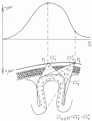Figure 8.1 This figure illustrates volume conductor theory for a cortical source that occupies a gyrus. The distribution of the amplitude of the voltage that reaches the scalp surface is shown in line S. The current that reaches the electrode from the cortical source is equivalent to the area contained by the lines that begin at the cortex and converge on the electrodes P1 or P2. For P1, the gyral convexity source projects only negativity. For P2, the source projects both negativity from the outer cortex and positivity from the inner cortex of the sulcus (shown by the area between the dashed lines that converge on P2). The cancellation effect of the inner cortex and the outer cortex (negativity added to positivity; the area within the dashed lines subtracted from that within the solid lines converging on P2) reduces the voltage of the signal detected by P2 as shown in line S. Although the figure is drawn in two dimensions, it is intended to represent three-dimensional space with the lines leading from the cortex to electrodes representing the sides of an approximately conical space. The amount of current reaching P1 and P2 then depends on the solid angle (signified by the omega characters in the figure) subtending the volume. (From Gloor P. 1985 Neuronal generators and the problem of localization in electroencephalography: application of volume conductor theory to electroencephalography. J Clin Neurophysiol. 2:327-354.)

The scalp EEG can be imagined as a constantly changing relief map in which the map is composed of hills and valleys whose height or depth represents a particular voltage that is determined by changing currents arising from underlying pyramidal cell postsynaptic potentials. Electrode placement is used to accurately map the contours of the changing voltages over the scalp surface. Each electrode, therefore, represents a spatial voltage sample point. The more electrodes used, the more faithfully they will map the actual contours of the scalp potentials. If too few electrodes are used, then the presence or absence of EEG changes in some areas of the scalp may be missed. This is somewhat analogous to digital sampling of EEG or audio signals. If too few samples are taken, then high frequency waveforms cannot be recorded. If too few electrodes are used, then voltage changes over areas in between will be completely missed. A certain number of electrodes is necessary to avoid spatial undersampling.

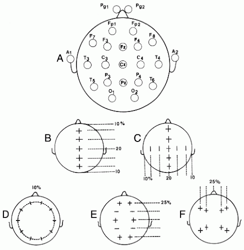Figure 8.2 This figure illustrates the steps outlined in the text (A through F) for measuring the head for the placement of the 10-20 system. (From Fisch BJ. Fisch and Spehlmann’s Digital and Analog EEG Primer. Amsterdam: Elsevier; 1999.)

Routine EEG recording uses 21 scalp electrode positions. These are placed according to the international 10-20 system of electrode placement described in Figure 8.2 (2). Although this is sufficient for routine clinical recording, to accurately sample the scalp surface for the detection of small signals generated by evoked potential recordings, or for research in quantitative EEG analysis and intracranial localization, it is estimated that at least 100 electrodes would be needed (3).

Spatial sampling in neonates also follows the 10-20 system, but because of the reduced head size fewer electrodes are used. F7, F3, F8, F4, P7, P3, P8, and P4 are excluded. Fp1 and Fp2 are replaced by more posterior electrodes, Fp3 located midway between Fp1 and F3 and Fp4 located midway between Fp2 and F4, consistent with the relatively more posterior location of the frontal lobes in relation to skull measurements at that age (4). If
A1 and A2 cannot be applied to the earlobe then the mastoid position is used (5).

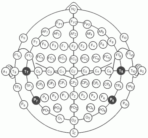Figure 8.3 The 10% system of electrode placement is shown, with T7, T8, P7, and P8 replacing the formerly named T3, T4, T5, and T6 electrodes to maintain naming consistency. The added electrodes at 10% distances are named according to the surrounding 10-20 electrodes. Note that in recording an anterior temporal source that FT9 and FT10 placement is usually superior to F7 and F8, which are located over the posterior lateral frontal lobes.

As illustrated in Figures 8.2 and 8.3, each recording electrode is named with a letter indicating the head region and a subscript number indicating the side of the head (odd numbers are left and even right) or z for the midline. The further the electrodes are placed laterally from the midline, the higher the subscript number (e.g., P7 is lateral to P3). Measurements of the head are made with a measuring tape (calipers or other methods should never be used). Measurements are all based on four landmarks: the nasion (lower forehead between the eyes), the inion (bone protruberance in the midline back of the head), and the left and right preauricular point (immediately anterior to the auditory canal). Measurements are made sequentially as shown in Figure 8.2 and summarized as follows:

The midline distance between the inion and nasion is measured. Beginning at 10% of the total distance above the inion (or nasion), a scalp mark is placed with a wax pencil. Then three more marks are placed at intervals of 20% of the total nasion to inion distance to establish the positions for Fz, Cz, and Pz.
The coronal distance between the left and right preauricular points intersecting with Cz is measured. Points at 20% and 40% of the total distance are then placed from Cz on the left and right to mark the positions for C3, C4, T7, and T8.
The distance around the head that passes through T7, T8, and the points 10% above the inion and nasion is measured by placing the measuring tape around the patient’s head. Once that measurement is obtained, Fp1 is placed at 5% of the total distance on the circumferential line to the left of the midline. Then marks are placed at intervals of 10% of the total distance around the head with the last mark at the Fp2 position. These marks establish the positions for F7, T7, P7, O1, 02, P8, T8, F8, and Fp2.
The front to back distance from Fp1 and Fp2 running through C3 and C4 to O1 and O2 respectively, is measured on each side. At half the distance between Fp1 and C3 on the left, and Fp2 and C4 on the right, F3 and F4 positions are marked, respectively. Similarly, the midpoints between C3 and O1 on the left, and C4 and O2 on the right give the positions for P3 and P4.
Next, the measurements are taken from F7 to F8 through Fz to define the transverse coordinates for F3 at the midpoint between F3 and Fz, and for F4 half way between Fz and F8. Similarly, measurements from T5 to T6 through Pz locate the transverse coordinates for P3 midway between T5 and Pz and for P4 midway between Pz and T6.

If an electrode cannot be placed (due to scalp defects, bandages, or monitors), then the nearest available electrode site of the “10-10” combinatorial system should be used, and the corresponding electrode on the other side of the head should be moved to the same mirror image position.

It should be kept in mind by the electroencephalographer that there is no substitute for the careful approach to measure the head outlined above. Unfortunately, it is also the procedure in which short cuts are taken by some EEG technologists. With the advent of digital EEG and video, it is reasonable to request that the technologist include the electrode measurement and application process in the video recording of each EEG as a quality control measure.

In some clinical situations (e.g., presurgical epilepsy monitoring), better localization may require using more than 21 electrodes. In such cases, selected additional electrodes are placed according to the 10-10 system described in Figure 8.3.

Physiologic electrical currents are detected using differential amplifiers. Each amplifier has two electrode inputs, named input terminal 1 and input terminal 2. The amplifiers subtract the voltage of the input 2 electrode from the input 1 electrode (input 1 input 2 = recorded EEG signal), hence differential amplification. Differential amplification is used for the recording of all bioelectrical signals (ECG, EMG, EEG). The advantage of differential amplifiers is that they cancel external noise. The most common sources of noise arise from other electrical devices. In environments where current is provided at 60 or 50 cycles/sec, the electrical interference nearly equally contaminates both input 1 and 2 electrode wires with 60 or 50 cycle signals. Because the differential amplifier subtracts the input 2 signal from the input 1 signal, the electrical interference that is equal in both inputs cancels out and is removed from the signal. However, because differential amplification is used, the absolute voltage value at electrodes attached to either input 1 or 2 is never known, only the difference between them is known. Fortunately, by comparing a number of electrode positions, the EEG can give a good approximation of the activity at a particular scalp location relative to other locations.

DIFFERENTIAL AMPLIFIER POLARITY

As noted above and illustrated in Figure 8.1, the currents flowing through the scalp have a polarity that is either positive or negative. The comparison of electrodes by differential amplification yields a difference in voltage and assigns the output a polarity (negative or positive). As described above, the signal output and its polarity are achieved by subtracting the voltages between input 1 and 2. The voltage is displayed on the EEG monitor or recording paper by the distance the signal deviates from the zero baseline. The polarity is displayed according to the direction the waveform deflects (above or below the baseline). If the voltage in the electrode in input 1 is —50 µV and the voltage in the electrode in input 2 is +50 µV, then the EEG signal will be input 1 minus input 2, or in this case (−50) — (+50) = —100 µV. In addition to knowing that input 1 is subtracted from input 2, the electroencephalographer has to understand how the amplifier orients the direction of the waveforms upward or downward to indicate the relative polarity of the signal.

As shown in Figure 8.4, the convention for biologic recording is that, if input 1 is more negative than input 2, the output signal will deflect upward, whereas if input 1 is more positive than input 2, then the output signal will deflect downward. This is the same as stating that if input 2 is more positive than input 1, then the signal will deflect upward, and if input 2 is more negative than input 1, then the signal will deflect downward. Also, if the polarity and voltage in the input 1 electrode is the same as in the input 2 electrode, then the output signal will be a flat line (zero).

Only gold members can continue reading. Log In or Register to continue