9 Basic Statistics for Electrodiagnostic Studies

For every electrodiagnostic (EDX) test performed, one needs to decide if the study is normal or abnormal. That determination often needs to be made in real time as the testing progresses, so that the study can be modified based on new information obtained as the testing proceeds. However, interpreting a test as normal or abnormal is not always straightforward, and requires some understanding of basic statistics. A full discussion of statistics is beyond the scope and purpose of this text, but there are some basic statistical concepts that every electromyographer needs to know in order to properly interpret a study.

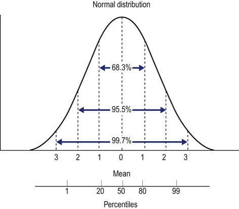
No two normal individuals have precisely the same findings on any biologic measurement, regardless of whether it is a serum sodium level, a hematocrit level, or a distal median motor latency. Most populations can be modeled as a normal distribution, wherein there is a variation of values above and below the mean. This normal distribution results in the commonly described bell-shaped curve (Figure 9–1). The center of the bell-shaped curve is the mean or average value of a test. It is defined as follows:

FIGURE 9–1 Normal distribution.

Many biologic variables can be modeled as a normal distribution wherein there is a variation of values above and below the mean. This normal distribution results in a bell-shaped curve. The center of the bell-shaped curve is the mean or average value of a test. The numbers on the x-axis represent the number of standard deviations above and below the mean. The standard deviation is a measure of the dispersion or variation in a distribution. The number of standard deviations above and below the mean define a certain portion of the population.

where x = an individual test result, and N = total number of individuals tested.

The standard deviation (SD) is a statistic used as a measure of the dispersion or variation in a distribution. In general, it is a measure of the extent to which numbers are spread around their average. It is defined as follows:

The reasons that the SD is such a useful measure of the scatter of the population in a normal distribution are as follows (Figure 9–1):

In EDX studies, one usually uses a lower or upper cutoff value, not both. For instance, a normal serum sodium may be 130 to 145 mmol/L (lower and upper cutoffs); however, a normal median distal motor latency is less than 4.4 ms (i.e., there is no lower cutoff because there is no median distal motor latency that is too good). Thus, for tests where the abnormal values are limited to one tail of the bell-shaped curve, instead of two:

These facts are important because cutoff values for most EDX studies often are set at 2 or 2.5 SD above or below the mean for upper and lower cutoff limits, respectively. After cutoff limits are established, one must next appreciate the important concepts of specificity and sensitivity of a test.

The specificity of a test is the percentage of all patients without the condition (i.e., normals) who have a negative test. Thus, when a test is applied to a population of patients who are normal, the test will correctly identify all patients as normal who do not exceed the cutoff value (true negative); however, it will misidentify a small number of normal patients as abnormal (false positive) (Figure 9–2, left). It is important to remember that every positive test is not necessarily a true positive; there will always be a small percentage of patients (approximately 1–2%) who will be misidentified.

FIGURE 9–2 Cutoff values and false results.

Left: When a test is applied to a population of normal patients, the test will correctly identify all patients who are below the cutoff value as normal (true negative [green in the figure]); however, it will misidentify a small number of normal patients who are above the cutoff value as abnormal (false positive [dark blue in the figure]). Right: When a test is applied to a disease population, the test will correctly identify all abnormal patients who exceed the cutoff value (true positive [red in the figure]); however, it will misidentify a small number of abnormal patients who are below the cutoff value as normal (false negative [dark blue in the figure]).

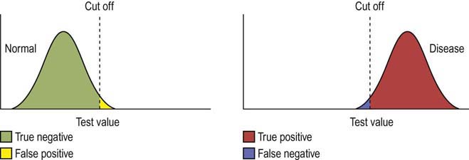
The sensitivity of a test is the percentage of all patients with the condition who have a positive test. When a test is applied to a disease population, the test will correctly identify all abnormal patients who exceed the cutoff value (true positive); however, it will misidentify a small number of abnormal patients as normal (false negative) (Figure 9–2, right). Thus, it is equally important to remember that every negative test is not necessarily a true negative; there will always be a small percentage of abnormal patients (approximately 1–2%) who will be misidentified as normal. Thus, the specificity and sensitivity can be calculated as follows:

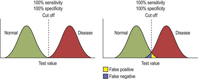
In an ideal setting, there would be no overlap between a normal and a disease population. Then, a cutoff value could be placed between the two populations, and such a test would have 100% sensitivity and 100% specificity (Figure 9–3, left). However, in the real world, there is always some overlap between a normal and disease population (Figure 9–3, right). If a test has very high sensitivity and specificity, it will correctly identify nearly all normals and abnormals; however, there will remain a small number of normal patients misidentified as abnormal (false positive) and a small number of abnormal patients misidentified as normal (false negative).

FIGURE 9–3 Selection of cutoff values.

Left: Ideally, there would be no overlap between a normal (green) and a disease (red) population, and the cutoff value could be placed between the two populations, yielding 100% sensitivity and 100% specificity. Right: In biologic populations, there is always some overlap between normal and disease populations. If a test has very high sensitivity and specificity, it will correctly identify nearly all normals and abnormals; however, there will remain a small number of normal patients misidentified as abnormal (false positive [yellow in the figure]) and a small number of abnormal patients misidentified as normal (false negative [dark blue in the figure]).

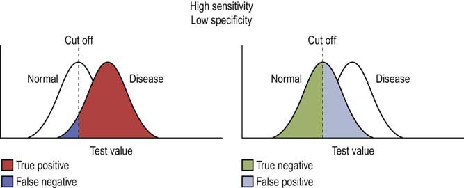
Often there is a compromise between sensitivity and specificity when setting a cutoff value. Take the example of a normal and a disease population where there is significant overlap between the populations for the value of a test. If the cutoff value is set low, the test will have high sensitivity but very low specificity (Figure 9–4). In this case, the test will correctly diagnose nearly all the abnormals correctly (true positive) and will only misidentify a few as normal (false negative) (Figure 9–4, left). However, the tradeoff for this high sensitivity will be low specificity. In this case, a high number of normal patients will be classified as abnormal (false positive) (Figure 9–4, right).

FIGURE 9–4 Advantages and disadvantages: high sensitivity and low specificity.

Left: If the cutoff value is set low (high sensitivity), the test will correctly diagnose nearly all the abnormals correctly (true positives [red in the figure]) and will misidentify only a few as normal (false negatives [dark blue in the figure]). Right: The tradeoff for this high sensitivity will be low specificity. In this case, some normals will be identified as normal (true positives [green in the figure]) but a high number of normal patients will be classified as abnormal (false positives [light blue in the figure]).

Related posts:

II: Polyneuropathy Anomalous Innervations Femoral Neuropathy Basic Nerve Conduction Studies Lumbosacral Plexopathy Routine Upper Extremity, Facial, and Phrenic Nerve Conduction Techniques

Stay updated, free articles. Join our Telegram channel

Join