Event-Related Potentials: General Aspects of Methodology and Quantification
Fernando H. Lopes Da Silva
Electroencephalography as a general method for the investigation of human brain function includes ways of determining the reactions of the brain to a variety of stimuli. Some of these reactions may be associated with clear-cut changes in the EEG; some others, however, consist of changes that are difficult to visualize. The research field dedicated to the detection, quantification, and physiologic analysis of those slight EEG changes that are related to particular events has steadily grown as a field of great interest in the last decades. These EEG changes may be treated globally under the common term event-related potentials (ERPs); a subset of the ERPs is sensory (visual, auditory, somatosensory) evoked potentials (ERPs). This chapter focuses on some general aspects of ERPs. Detailed descriptions of specific aspects of ERPs to stimuli of different modalities are presented in separate chapters (visual in Chapter 46, auditory in Chapter 47, and somatosensory in Chapter 48), as well as general aspects of event-related (des)ynchronization in Chapter 45. Specialized aspects of ERPs of children and infants are presented in Chapter 49 and the use of ERPs in the operating room is covered in Chapter 38.
Regan published an authoritative specialized textbook on this topic in 1972 and a thorough revised form in 1989; other early general sources include Storm van Leeuwen et al. (1), John and Thatcher (2), Callaway et al. (3), Barber (4), Chiappa (5), and Misulis and Fakhoury (6). Reviews of the applications of computer methods to ERP detection and analysis are those of Barrett (7), Gevins and Cutillo (8), and Regan (9). Insightful accounts of steady-state (10) and transient evoked potentials (11) are presented in the book edited by Nunez Neocortical Dynamics and Human EEG Rhythms (10).
EVOKED-RELATED POTENTIAL ANALYSIS: GENERAL ASPECTS
ERPs are usually defined in the time domain as the brain electrical activity that is triggered by the occurrence of particular events or stimuli. A basic problem of analysis is how to detect ERP activity within the often much larger ongoing EEG or background activity (i.e., the activity not related to the stimulus). Dawson (12), a pioneer in the field, attempted first to solve this problem by the photographic superposition on the screen of an oscilloscope of a number of time-locked responses. This method had the property of enhancing response in contrast to the ongoing activity while providing, at the same time, an indication of response variability. It is, however, difficult to quantify the results in this way. Since the introduction of the summation method (13) and the development of digital computer techniques (14, 15 and 16), ERPs are obtained in special-purpose digital computers and expressed as time-varying functions. In general terms, there is no fundamental argument to justify the preference for either time or frequency ERP analysis. Both reflect the same reality. The choice of analytic domain, therefore, is determined by practical considerations. Nevertheless, a certain model of the generation of ERPs is always implicit in the choice of a method of analysis of these potentials.
BASIC MODELS OF ERPS
According to the most widely accepted model, ERPs are signals generated by neural populations that are time-locked to the stimulus; these signals would be summed to the ongoing EEG activity. According to another model, however, ERPs are assumed to result, at least partially, from a reorganization of the ongoing activity. This view arose from the seminal work of Sayers et al. (17) who analyzed segments of EEG recorded before and immediately after the presentation of auditory stimuli. They carried out a Fourier analysis computing the real and imaginary coefficients of the signal’s frequency components. In this way they constructed amplitude and phase spectra, and found that the brainstem-evoked potentials (BAEPs) to auditory stimuli could be distinguished much better using the distributions of phase spectral values, rather than the distributions of amplitude values. In a later study McClelland and Sayers (18) showed further that the magnitude of the differences between amplitude spectra of pre- and post-stimulus epochs decreased progressively as stimulus intensity was reduced. Examining separately amplitude and phase spectra of the response ensemble, these authors showed that the phase standard deviation for responses at auditory threshold was generally significantly smaller than for the corresponding harmonics obtained from subthreshold responses. In contrast, the amplitude differences between populations of threshold and subthreshold responses were generally non-significant. These findings led the authors to conclude that the use of BAEPs for auditory threshold determination should preferentially be based on ensemble phase measures rather than amplitude measures.
These experimental results indicate that the brain response to a stimulus may consist, at least partially, of a decrease of phase variance of certain frequency components, that is, an enhanced alignment of the phase components of ongoing EEG or MEG signals, or phase resetting.
More recently Makeig et al. (19) demonstrated that ERPs could be generated by stimulus-induced phase resetting of ongoing EEG components. Mazaheri and Picton (20) showed, by subtracting the spectra of the average ERP from the average spectra of single trials, that ERPs can involve phase resetting of the ongoing EEG rhythms. Nonetheless, Mäkinen et al. (21) argued that a high degree of independence exists between ongoing brain activity and auditory ERPs, and suggested to use amplitude variance to distinguish whether or not phase resetting is present in an ERP. An unambiguous assessment of phase resetting, however, implies a measure of variance of phase values and cannot be based just on amplitude variance, as appropriately pointed out by Klimesch et al. (22).
This issue was addressed by Mazaheri and Jensen (23) in an interesting way; they introduced a measure—the phase preservation index—to compare quantitatively the phase of alpha oscillations before and after a visual stimulus. The main finding was that the alpha oscillations preserve their phase relationship with respect to the phase before the stimulus, and their conclusion was that different neuronal populations appear to generate the ongoing oscillations and the ERPs, but this does not imply that the neuronal populations are macroscopically distinguishable.
An underlying problem, however, is the fact that in all these cases of event-related responses the signal-to-noise ratio plays a fundamental role. The original findings of Sayers et al. (17) that the phase spectrum was more powerful than the amplitude spectrum in distinguishing auditory ERPs were obtained at very low stimulus intensities, that is, at the threshold for auditory discrimination. This is not the case in many other experiments. In a recent overview of this issue we (24) proposed that it is likely that the relative amount of phase preservation from the pre- to the post-stimulus epochs will depend on several factors; at least four appear to be particularly relevant:
the baseline level of the ongoing oscillations,
the frequency band of the oscillations,
the stimulus modality and its strength, and
the specific cortical area, since EEG rhythmic activities are not equally distributed over the cortex.
Moreover, it is important to note that a solution to this question may not be resolved using only scalp EEG/MEG records, as also stated by Mazaheri and Jensen (23) who propose that intracranial recordings will be necessary, combining single cell and local field potential recordings with EEG signals.
We may state from a theoretical point of view that it is not probable that two independent neuronal populations, one generating exclusively ongoing activity and another one responsible for the evoked response, would exist side by side as distinct entities in a given brain area. It is more likely that the same neuronal elements are involved in the generation of both types of signals but working in different modes. This same idea was formulated by Shah et al. (25) who noted that EEG ongoing activity and ERPs are generated by overlapping neuronal elements. According to this model, ERPs may engage a group of neurons, by way of two basic mechanisms: either by enhancing the synchrony of increases, or decreases, of neuronal firing rates and/or by synchronized membrane transients or oscillations. These two mechanisms are not mutually exclusive. It follows that the former mechanism will lead to changes of amplitude, but this will also be the case for the latter, since the activity of those neurons that work synchronously in phase corresponds to larger amplitude at the level of the population than that of neurons that display a random, or weak, alignment of phases. This reinforces the conclusions that amplitude variance is not sufficient to determine whether phase resetting occurs in event-related responses. In any case, the assessment of phase resetting needs the direct estimation of phase variance of frequency components. This means that, in the most general case, the analysis of event-related EEG/MEG changes of activity should take into consideration not only spectral amplitude, but also phase. In this respect, it is also interesting to note that recently more attention is being put on the use of the imaginary part of coherency, which in fact constitutes the phase spectrum, to analyze interactions between different EEG signals (26).
Notwithstanding the importance of phase in the generation of ERPs in general, the wide use of time averaging of ERP amplitude waveforms in practical ERP work is so overwhelming that this form of analysis is treated first in the following section. After that we consider analyses in the frequency domain and lastly analyses according to integrated time-frequency approaches.
TIME AVERAGING OF ERPs
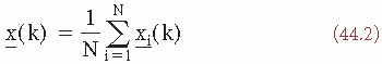
According to the classic view, ERP analysis is based on two basic assumptions: (i) the electrical response evoked from the brain is invariably delayed relative to the stimulus and (ii) the ongoing activity is a stationary noise, the samples of which may or may not be correlated. In this way, ERP can be considered a signal (s(k)) corrupted by additive noise (n(k)), the ongoing activity. (Assume that the signals are sampled, with k as the discrete time variable.) ERP detection becomes, in this way, a question of improving signal-to-noise ratio. In the more general and simplified case one assumes a simple additive model (stochastic variables are indicated by underlined symbols). The recorded stochastic signal x(k) is given as a sum of two terms:
The expected value of n(k) is zero. The average of x(k) over N realizations is then defined as:
The expected value of the average is given as:
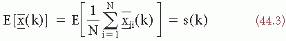
[since E(n(k))] = 0. The variance of x(k) is as follows:
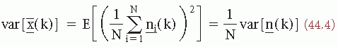
since s(k) is assumed to be invariant. Therefore, the signal-to-noise ratio in terms of amplitude improves proportionally to  . In more general terms, however, it should be assumed that the signal s(k) is a stochastic signal, so that expression 44.1 should be reformulated as follows:
. In more general terms, however, it should be assumed that the signal s(k) is a stochastic signal, so that expression 44.1 should be reformulated as follows:The importance of this apparently small difference lies in the fact that the model given by expression 44.5 implies that the EP is not fully described by the mean value of x(k), but also by the higher statistical moments, as, for instance, the variance. In most practical cases, the latter model (expression 44.5) gives a better account of reality. As pointed out by John et al. (27), the former model (expression 44.1) is valid only for anesthetized preparations and possibly for the short-latency components of EP that mainly reflect sensory processes; this is, however, not the case for long-latency components.
For a comprehensive study of EP, multivariate analysis methods may be used (28, 29, 30 and 31). In this case, one considers an EP to be a multidimensional stochastic variable, that is, a vector x where the elements are the values in subsequent time points:
Thus, the expression 44.5 can be rewritten as a vectorial sum:
assuming that E(n) = 0 as before. Therefore:
The second-order moment of × is given by the covariance matrix C; considering any two samples represented by k and 1, one may write:
There are multivariate statistical methods that enable the structure of such signals as EPs to be represented as functions of a small number of factors. A technique to achieve this form of representation is the principal components method. The essence of the principal components method is to account for the EP as a linear combination of a small number of basis functions. It can be proved (e.g., Ref. 32) that, if one chooses as basic functions the eigenfunctions ψi, of the covariance matrix, the following expression gives the best p-dimensional approximation (in a least-squares sense) to the EP (P < NS):
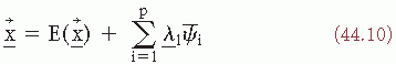
In the expression, the coefficients  are uncorrelated and the eigenfunctions ψ1 are orthogonal. It should be noted, however, that this form of description is only a statistical way of describing EP; one cannot assume that the eigenfunctions necessarily correspond to independent physiologic generators (33). Nevertheless, the method can be very useful for data reduction in EP research where one wants to go further than the mean value of the EP.
are uncorrelated and the eigenfunctions ψ1 are orthogonal. It should be noted, however, that this form of description is only a statistical way of describing EP; one cannot assume that the eigenfunctions necessarily correspond to independent physiologic generators (33). Nevertheless, the method can be very useful for data reduction in EP research where one wants to go further than the mean value of the EP.In principal components analysis, the first component is the one accounting for the greatest variance; as many components as one wishes can be determined in order to account for a certain percentage of the total variance. In EP analysis, it is usually not necessary to go further than i = 4 or 5. In this way, a parsimonious description of EP can be achieved. Principal components analysis, however, is no more than a transformation of the original data. In this form of analysis, no provision can be made for variance components attributable only to the unreliability of the observations (32). This and other shortcomings of principal components analysis can be solved by way of the mathematical model of factor analysis.
In factor analysis, each observation xi is represented in terms of a linear function of common factor variables and of a signal latent-specific variable that can be represented as follows (provided that the means of the observations are zero):
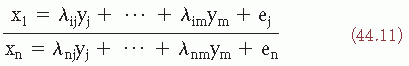
where yj is the jth common factor variable, λij is called the loading of the ith observation on the jth common factor, and ei is the ith specific factor variable. The covariances of the observations xi are reflected only on the specific factors. Factor analysis is based on a specific statistical model in which the number of common factors is specified beforehand; an example of factor analysis in EP research is shown in Figure 44.1. These methods of analysis can be of great usefulness in order to provide a small set of features that can be employed for the classification and clustering of EP as discussed below (28,34, 35, 36 and 37). As an illustration of the usefulness of principal components and discriminant analysis, the study of Donchin and Cohen (38) found that the discriminant between EP recorded to task-relevant and task-irrelevant stimuli was based essentially on time points at 300 msec.
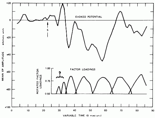 Figure 44.1 Average evoked potential (ERP) of one subject (parietal leads; N = 512 epochs; epoch length, 765 msec) and the corresponding seven factor loading plots. The reality of the first two factors in the waveform of this example is questionable, because the factors also showed loadings in the prestimulus period. (Adapted from Rebert CS. Neuroelectric measures of lateral specialization in relation to performance. Electroencephalogr Clin Neurophysiol. 1978;34:231-238.) |
Another form of data reduction of average EP involves describing EP as a sum of a set of analytic functions, such as damped sinusoids as thoroughly investigated by Freeman (39,40). Later, this chapter discusses the possibility of describing EP as a sum of harmonically related sine waves (i.e., Fourier components).
SPECIAL PROBLEMS IN ERP TIME AVERAGING
ERPs in Strong Rhythmic Background EEG
One problem is whether the statistical properties of the background activity may have influence on the degree of improvement regarding signal-to-noise ratio realized by the averaging procedure. In detecting ERPs by classic time averaging, the main objective, of course, is to increase the signal-to-noise ratio so that the EEG background activity will be attenuated. Equation 44.4 illustrates that the ratio between the variance of the averaged signal and the variance of the noise is 1/N. This holds for the case where the noise samples are uncorrelated. Often, however, this is not the case, as, for instance, in the presence of a strong rhythmic background such as an alpha rhythm. In such a case, subsequent samples of n(k) are not independent. The degree of dependence of the samples of n(k) is given by the autocorrelation function of the background activity (see for a definition Chapter 54).
Assuming that σ2 is the var[n(k)], the ERP variance [var(x(k))] is not equal to [1/N(var(n(k)))], as in Equation 44.4, but equal to [σ2/N(var(n(k)))] multiplied by a factor that depends on the properties of the autocorrelation function of the background activity (41). It is therefore important to emphasize that rhythmicity of the background can influence the signal-to-noise ratio. McGillem and Aunon (42), Steeger (43), and Steeger and Reinhardt (44) described methods that can provide better estimates of average ERP because they take into account the statistical properties of the ongoing EEG activity.
A related problem is whether the stimulation should be periodic or aperiodic; aperiodic stimulation can lead to reduced ERP variance as shown theoretically by Ten Hoopen (45) and experimentally by Arnal and Gerin (46). More specifically, Ruchkin (47) has demonstrated that the variance of the averaging estimate is closer to zero when the interstimuli intervals are exponentially distributed (Fig. 44.2).
Single-Trial ERPs and Classification
In the last decades there have been several studies with the aim of identifying single-trial ERPs and/or to discriminate subgroups of ERPs among a series of trials. Initially most of the approaches applied were based on cross-correlation of EEG signals, including the ERP, and some template a priori determined (42,48), and on maximum likelihood detectors (49). According to one of these methods (44), a matched filter is created that is adapted optimally to the template (the average ERP) as well as to the actual ongoing activity, which is estimated by its autocorrelation function (Woody’s adaptive filter was only adapted optimally to the template and to white noise). Each single-trial EEG segment is then passed through the matched filter and the maximum output signal is found; in this way an optimal average ERP can be obtained after correction for latency deviations. A method related to those described above but also involving a classification process was proposed by Pfurtscheller and Cooper (50) under the term selective averaging; according to this technique, single-trial ERPs are cross-correlated with different templates. The maxima of the cross-correlation functions are used to estimate the amplitude and latency of particular components. Thereafter, those trials that fall within certain amplitude and/or latency limits are averaged. In this way, different types of selected averages can be obtained that may correspond to different subsystems and/or physiologic conditions. In cases where all trials are averaged together, there is a considerable information loss. The problem of measuring single-trial ERPs has been extensively investigated by Coppola et al. (51). In this study, equations have been proposed to estimate empirically
S/N that may be useful in ERP clinical or psychophysiological studies (for details see Ref. 51).
S/N that may be useful in ERP clinical or psychophysiological studies (for details see Ref. 51).
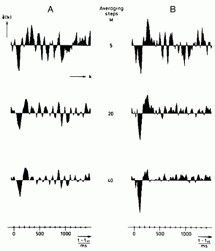 Figure 44.2 Average ERPs recorded between vertex and mastoid; stimulus is a sinusoidal tone of 1000 Hz, 40 dB above 2104 µbar, 600 msec. A: The results of simple averaging are shown for a number of averaging steps. B: The results obtained using an adaptive filter (based on a maximum likelihood detector adapted to broadband colored noise) followed by synchronization and averaging are shown. Note the improvement in ERP discrimination. The plots are in relative vertical scale; tst is the stimulus onset. (Courtesy of G.H. Steeger.) |
The analysis of single-trial ERP is also important in determining whether a certain single-trial ERP belongs to a specific ERP class. This problem of classification can be solved using multivariate statistical methods (34). In general terms, the question involves: (i) describing ERP by a set of features (in the simplest case, the values of the sample points) and establishing a feature profile, (ii) making a learning set where ERPs corresponding to a priori defined classes are pooled, and (iii) finding a discriminant function (i.e., a decision rule) that must partition the space occupied by all objects (the ERP) so that unique patterns corresponding to different classes can be identified. (iv) Finally, the class to which any new object (i.e., a single-trial ERP) belongs must be determined; this is accomplished by computing a discriminant score for each object. Thus, each single-trial ERP is classified in the subspace within which the discriminant score falls. The ERP features used in the procedure can be simply the corresponding sample values or a reduced amount of data, such as can be obtained using factor or principal component analysis.
Related posts:

Stay updated, free articles. Join our Telegram channel

Full access? Get Clinical Tree


