Magnetoencephalography: Methods and Applications
Riitta Hari
Recording of weak magnetic fields outside the head by means of magnetoencephalography (MEG) emerged in the late 1960s, 40 years after the invention of the human EEG. The first instrument was an induction coil magnetometer with 2 million turns of wire. It was used to detect the magnetic alpha rhythm by means of signal averaging, with the electric alpha as the time reference (1). The MEG method became more practical with the introduction of SQUID (superconducting quantum interference device) magnetometers in the early 1970s; since then it has been possible to record both spontaneous and evoked magnetic signals of the human brain without any EEG reference. Rapid development of the technology has taken place during the last few years: sensor arrays with whole-scalp coverage are now commercially available, and signal analysis methods have progressed quickly. At present, tens of laboratories worldwide utilize MEG for exploration of normal and abnormal functions of the human brain, and MEG results continue to influence interpretation of EEG data.
In this chapter, the basic principles of MEG are reviewed briefly, with examples mainly from our own laboratory. Both spontaneous and evoked activities in normal subjects and in some neurologic patients are discussed to the extent which is supposed to be of immediate interest to a clinical neurophysiologist. Several review articles are available for consulting MEG findings directly related to basic brain research and relevant methodology (2, 3, 4, 5, 6, 7, 8, 9, 10, 11, 12, 13, 14, 15, 16, 17 and 18). The main advantages of MEG are its good spatial resolution in locating cortical events and its selectivity to activity of the fissural cortex. The sites of active brain areas can be located with respect to external landmarks on the head, brain structures, or functional brain regions (identified by means of sources of evoked responses).
One goal of MEG recordings is to obtain information about the neural generators of various signals. The EEG research has traditionally focused on temporal waveforms, and a whole branch of electrophenomenology has arisen around EEG “graphoelements,” which have been correlated with different tasks and stimulation parameters, clinical states, and even with personality factors. It is clear that a better understanding of the generators underlying the EEG signals would permit a more precise and physiologic interpretation of abnormalities. MEG has considerably clarified these issues during the last decade, both at conceptual and practical level, and may have much to offer in the future.
COMPARISON OF EEG AND MEG
MEG is closely related to EEG. Despite different sensitivities of EEG and MEG to sources of different orientations and locations, the primary currents causing the signals are the same. Similarities between the MEG and EEG waveforms are therefore to be expected. The advantage of MEG over EEG in source identification results mainly from the transparency of the skull and other extracerebral tissues to the magnetic field, in contrast to the substantial distortion and smearing of the electric potentials. Thus the MEG pattern outside the head is less distorted than the EEG distribution on the scalp. The magnetic recording is also reference-free, whereas the electric brain maps depend on the location of the reference electrode. As a result it is often difficult to make a reasonable guess of the source locations by visual inspection of the EEG data. Reference-free EEG presentations can be obtained by calculating the “surface Laplacians” (19,20). However, even then one has to proceed to neural sources for proper interpretation, and problems arise for several simultaneous source. The Laplacians cannot be calculated for the outermost electrodes, which reduces the brain areas that can be characterized.
Figure 42.1 shows a current dipole in a spherical volume conductor consisting of four layers of different conductivities that simulate the brain, the cerebrospinal fluid, the skull, and the scalp. The resulting distributions of electric potential and magnetic field are “dipolar,” that is, display two extrema of opposite polarities, but rotated by 90° with respect to each other. The isocontour lines are relatively more tight in the magnetic than in the electric pattern because concentric electric inhomogeneities smear only the electric potential, while the magnetic pattern is not influenced. In an ideal sphere, a single superficial tangential dipole can be found one third more accurately on the basis of magnetic than electric recordings (21). For interpretation of MEG signals recorded from the real brain, it is sufficient to use a realistically shaped model consisting of the brain only, while accurate EEG calculations require a full multicompartment model with known conductivities and shapes for the brain, skull, cerebrospinal fluid, and scalp.
MEG’s selectivity to tangential currents in the presence of several simultaneous sources is an important advantage in practical work, as is illustrated, for example, by the early differentiation between multiple cortical areas activated by somatosensory stimuli (12,22, 23, 24, 25 and 26). Moreover, it is often more straightforward to interpret MEG than EEG data.
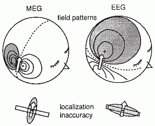 Figure 42.1 Magnetoencephalographic (MEG) and electroencephalographic (EEG) field patterns over a concentric four-layer sphere when a tangential current dipole (shown by the arrow) is active in an area approximating the second somatosensory cortex in the upper lip of the Sylvian fissure. The shadowed areas indicate the magnetic flux out of the head (MEG) and positive potential (EEG). The lower part of the figure illustrates schematically, with shadowed ellipsoids, the inaccuracy region of the dipole location when computed “backwards” from the signals on the surface. The dipole is assumed to be in a wall of a cortical fissure. |
Since both electric and magnetic signals are generated by the same primary currents that flow in the brain and the nearby tissues, one should pay attention to both MEG and EEG data when drawing conclusions on brain function from either type of recordings. For example, a dipolar potential distribution could be explained equally well with two radial current dipoles or with one tangential dipole. However, the existence of a clear magnetic pattern, rotated 90° with respect to the electric one, implies that the latter explanation should be favored (27). The minimum requirement for sound data interpretation is that the conclusions based on EEG and MEG do not contradict.
Some current sources (very deep and radial) are more reliably picked up by EEG than MEG, but MEG counterparts of auditory brainstem responses can be detected with MEG as well and they can give important information about the source configuration (28). However, the contribution of even deep activity to the MEG signals can be probed by inserting sources to interesting brain structures (such as thalamus or hippocampus) and then calculating the best fit of these sources, as a function of time, to the measured signals (29,30). In theory, current loops are electrically silent but magnetically visible. In practice, however, ideal current loops have not been observed, and all cerebral currents that give rise to MEG signals are also expected to generate electric potentials on the scalp. For maximum information, the MEG and EEG techniques should be combined, and the simultaneously recorded data should be interpreted with methods that take advantage of the complementarity of the records (see also the section “The contribution of neuronal models: in vitro and computational models” in Chapter 5).
MEG INSTRUMENTATION
The magnetic field generated by cerebral currents is two orders of magnitude weaker than that produced by the heart and only a tiny part of the steady magnetic field of the earth (Table 42.1). To avoid external magnetic artifacts caused by moving vehicles, power lines, radio transmission, and so on, it is common to carry out the recordings within a magnetically shielded room, usually made of several layers of aluminum and mu-metal. Biomagnetic measurements can also be performed without magnetic shielding when special compensation techniques are available. In general, it is however better to prevent than to compensate for artifacts. Adequate magnetically shielded rooms are commercially available.
Figure 42.2A gives a schematic illustration of, now already old-fashioned, arrangement during the MEG recording. The subject lies in a magnetically shielded room and the neuromagnetometer, containing SQUID sensors immersed in liquid helium (at -269°C), is positioned close to the head. To replace the evaporating helium, the Dewar container has to be refilled regularly, in modern devices about once a week. During recordings with the present-day devices that cover the whole scalp in a helmet-shaped array, such as the 306-channel neuromagnetometer in Figure 42.3, the subject is typically sitting during the measurement.
The cerebral magnetic field is coupled into the SQUID sensors through superconducting flux transformers. The transformer configuration is important for the device’s sensitivity to different source current configurations and to artifacts. A magnetometer, containing a single pick-up loop in the flux transformer, is most sensitive to signals but also to artifacts (Fig. 42.2C). A more elaborate axial first-order gradiometer contains a compensation coil, wound in the direction opposite to the pickup coil (Fig. 42.2B,C); this
configuration decreases the influence of distant disturbances that link the same magnetic flux into both coils. Therefore, the output of the axial first-order gradiometer is essentially determined by the signal of the nearby neuronal source itself. Furthermore, since the distance between the pickup and compensation coils of a first-order axial gradiometer is several centimeters, the measured signal approximates the amplitude of the radial field component Br rather than its axial derivative. Higher-order gradiometers are necessary for measurements performed without a magnetic shield; in these systems the sensitivity is reduced to the distant artifacts but to some extent also to the nearby brain currents.
configuration decreases the influence of distant disturbances that link the same magnetic flux into both coils. Therefore, the output of the axial first-order gradiometer is essentially determined by the signal of the nearby neuronal source itself. Furthermore, since the distance between the pickup and compensation coils of a first-order axial gradiometer is several centimeters, the measured signal approximates the amplitude of the radial field component Br rather than its axial derivative. Higher-order gradiometers are necessary for measurements performed without a magnetic shield; in these systems the sensitivity is reduced to the distant artifacts but to some extent also to the nearby brain currents.
Table 42.1 Orders of Magnitude of Magnetic Fields (in femtotesla, fT = 10-15 T) | ||||||||||||||||
|---|---|---|---|---|---|---|---|---|---|---|---|---|---|---|---|---|
| ||||||||||||||||
 .
.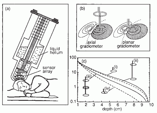 Figure 42.2 (A) Magnetoencephalogram recording. The subject is lying in a magnetically shielded room with his head supported by a vacuum cast. The Dewar containing the SQUID sensors is brought as close to the head as possible, without direct contact, and the magnetic field (or its gradient) is picked up outside the head at several locations simultaneously. (B) Two flux transformer configurations. The first-order axial gradiometer (left) measures essentially Br and detects the maximum signals at both sides of the dipole. The planar gradiometer (right) measures the tangential derivative  Br/ Br/ x or x or  Br/ Br/ y; the maximum signal is detected just above the dipole. (C) Dependence of signal strength (in arbitrary units) on the depth of a current dipole when measured by (i) a magnetometer, (ii) a first-order axial gradiometer, (iii) a second-order axial gradiometer, and (iv) a planar figureof-eight gradiometer. Simulations in a sphere of 10-cm radius. y; the maximum signal is detected just above the dipole. (C) Dependence of signal strength (in arbitrary units) on the depth of a current dipole when measured by (i) a magnetometer, (ii) a first-order axial gradiometer, (iii) a second-order axial gradiometer, and (iv) a planar figureof-eight gradiometer. Simulations in a sphere of 10-cm radius. |
The contour plots in Figure 42.2B illustrate the pattern of Br, the magnetic field radial to the surface, generated by a tangential current dipole in a sphere. The signal strengths measured with an axial gradiometer form a spatial pattern similar to the field itself, with extrema of opposite polarities at the two sides of the dipole. In contrast, the planar gradiometer yields the maximum signal when centered just over the dipole at the location of the steepest field gradient. The planar gradiometer is able to detect the location of the source even at the edge of the sensor array and the essential information from the field pattern can thus be obtained from a rather small measurement area. On the other hand, information about the depth of the source is more accurate with axial than planar sensors since the gradient decreases relatively more rapidly as the function of source depth than does the field itself (Fig. 42.2C). However, whole-scalp sensor coverage largely counterbalances this drawback. Although the patterns measured by both axial and planar gradiometers are easily interpreted, in practice it is often useful that the maximum signal detected by the planar gradiometers suggests the approximate source location. Methods have been developed to present data measured with different coil configurations in a standard format (31). On the basis of axial gradiometers, some users compute virtual planar gradiometer signals that work well as indicators of the most likely source areas but have ( times) more noise than the original signals.
times) more noise than the original signals.An essential part of the measurement system is the head-position indicator, which gives the exact measurement sites and the orientations of the sensors with respect to the head. We obtain this information by placing three to four small wire loops on known sites on the scalp. The field pattern produced by currents led through the loops is then measured with the multichannel magnetometer. In another commonly used head-position indicator system a transmitter is connected to magnetic sensors, which are fixed on the dewar, and three receivers are placed on the subject’s head. The head-position indicator devices allow the position of the magnetometer to be determined with respect to external landmarks on the head with 2- to 3-mm accuracy. The coordinate system is preferably global, typically fixed on the basis of the nasion, inion, and the preauricular points so that it can be easily transported to, for example, Talairach space commonly used in functional magnetic resonance imaging (MRI). The important landmarks on the head and the shape of the skull can be determined with a three-dimensional digitizer.
To determine the current distribution within the head, the magnetic field must be sampled at several locations, preferably simultaneously. When only single-channel magnetometers were in use, it sometimes took several days to complete a field map. For example, the MEG recordings of the first epileptic patients lasted for 16 hours (32)! Changes in the subject’s attentive state and vigilance were thus unavoidable. With the present-day helmet-shaped neuromagnetometers that cover the whole scalp
(Fig. 42.3), the whole field pattern can be measured without moving the instrument. This progress of instruments has finally made MEG recordings feasible for comprehensive studies of integrative brain functions in health and disease.
(Fig. 42.3), the whole field pattern can be measured without moving the instrument. This progress of instruments has finally made MEG recordings feasible for comprehensive studies of integrative brain functions in health and disease.
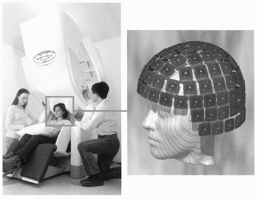 Figure 42.3 A modern 306-SQUID neuromagnetometer used in our laboratory. Each of the 102 three-channel sensor elements comprises two orthogonal planar gradiometers and one magnetometer; the helmet-shaped arrangement of the elements is shown on the right (courtesy of Mika Seppä). The planar flux transformers measure the tangential derivatives  Br/ Br/ x and x and  Br/ Br/ y of the radial field component Br. y of the radial field component Br. |
The optimal spacing of the sensors is determined by the spatial frequency of the signal distribution and, therefore, only marginal benefit can be obtained by reducing the sensor spacing below the distance between the source and the sensor, that is, about 3 cm (33,34). Thus about 150 sensors would suffice to cover the whole cortex, and the newest instruments with 200 to 300 sensors provide dense-enough spatial sampling for MEG recordings. The diameter of the sensor coil is always a matter of compromise: the larger the coil, the more sensitive it is, but also the more it averages the magnetic field, thereby leading to loss of information.
Currenlty (in 2010) about 140 whole-scalp neuromagnetometers are in use in clinical and research settings all over the world. The devices of different manufacturers vary in the number of channels, in the pickup coil configuration (e.g., first-, second-, or third-order axial gradiometer, planar gradiometer, or magnetometer), as well as in the area covered by the sensor array. However, the different devices provide practically very similar information about the brain’s neuronal currents.
With the present technology, the intrinsic noise of the SQUID is no longer a problem, and the main “noise” arises from the brain itself. Taking into account the distance of the coils from the source, pickup coils with diameters around 2 cm are reasonably sensitive and do not lose significant information. Decreasing the distance to the source improves the resolution of the system. Thus it would be important to develop flux transformer arrays that can be put close to the scalp of each subject, independent of the head shape. Such systems could be made with high-Tc superconductor arrays that require less insulation. However, despite the promising recordings of MEG signals with a single-channel high-Tc neuromagnetometer (35), the technique has not developed during the last years. The main reasons are the higher (thermal) noise of the sensors and the difficulty to easily manufacture multichannel high-Tc sensor arrays.
SOURCE IMAGING
Since the aim of MEG studies is to obtain information about brain function, the field pattern should be interpreted in terms of cerebral currents. Yet, due to the nonuniqueness of the inverse problem—namely that several current distributions can, in principle, produce identical magnetic field patterns outside the head—the interpretation usually requires the use of specific source and volume conductor models. Thus the situation is more complicated than in MRI, functional magnetic resonance imaging (fMRI), or in positron emission tomography (PET), where the inverse problem can be solved uniquely. However, physiologically meaningful solutions of MEG patterns can be found by utilizing constraints based on the known anatomy and physiology of the brain.
CURRENT DIPOLE
The most commonly used source model in MEG studies is a current dipole within a sphere. The dipole can be characterized by means of five parameters, three for its three-dimensional location, one for its orientation (only the plane parallel to the surface of the sphere is relevant), and one for its strength. In a sphere, only primary currents tangential to the surface will produce a magnetic field. In reality, signals may also be detected from the convexial cortex where the currents are considerably closer to the detector than are the currents within the wall of a fissure. Deviation of the convexial source by only 10 to 20 degrees from the radial orientation is enough to give a signal as large as that produced by a tangential dipole of the same size but 2 cm deeper in the fissural cortex. It therefore seems probable that under realistic conditions nearly radial sources may contribute significantly to the MEG signals. This notion is supported by simulations that took into account the real geometry of the cerebral cortex (38). A practical example of the possibility to detect tilted currents is the identification of magnetic counterparts of the P22 and P25 somatosensory responses, which are believed to arise in the convexial cortex (39, 40 and 41).
In dipole modeling, the location of the “equivalent current dipole” (ECD) is found by a least-squares fit to the data, typically at a time point of a clearly dipolar field pattern. In progressing toward a multidipole model, one may extract the field patterns produced by the already identified sources to facilitate further analysis (42, 43 and 44). The success of dipole models in MEG interpretation derives, in part, from the difficulty to discern the details of the brain activation pattern from the typical measurement distance of at least 3 cm from the source (Fig. 42.4). Consequently, a single current dipole is a reasonably accurate description of a local active cortical area of less than 2 to 3 cm in diameter.
The adequacy of the model can be evaluated by calculating the goodness-of-fit (g) value (5,45), that is the squared correlation coefficient between the measured signals and those predicted by the model. The g-value, however, depends on several factors such as the number and distribution of the measurement locations (46). A low g-value means that either the brain source significantly deviates from the model or that the signal-to-noise ratio is poor. It is also often useful to study the residual field, that is, the difference between the measured field and that predicted by the model, or to compare the waveforms predicted by the model with the measured waveforms. If the residual field shows systematic features that cannot be explained by noise, a different source configuration must be considered.
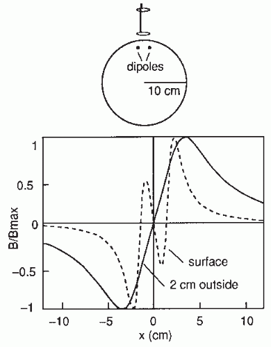 Figure 42.4 The dependence of the radial component of the magnetic field on the distance between the source and the detector. Two current dipoles are situated in a homogeneous sphere (radius 10 cm), 1 cm beneath the surface, 3 cm from each other, and symmetrically with respect to the origin. The field was calculated on an arc perpendicular to the orientation of the dipoles (x-axis). The pattern is complicated on the surface, whereas 2 cm outside the sphere the higher spatial frequencies have faded away and the dipolar term dominates. The amplitudes have been normalized according to the maximum value; the maximum field would be about seven times stronger on the surface than 2 cm above it. (Adapted from Hari R. Interpretation of cerebral magnetic fields elicited by somatosensory stimuli. In: Basar E, ed. Springer Series of Brain Dynamics. Berlin/Heidelberg: Springer-Verlag; 1988:305-310.) |
The inaccuracy of MEG localization is smallest in the direction transverse to dipole orientation (cf. Fig. 42.1) and largest (about double) in the direction of depth. The locating accuracy depends drastically on the signal-to-noise ratio, which is improved by signal averaging for evoked responses but cannot be affected much—except by filtering—in the case of spontaneous activity. For comparison, note that the best localization accuracy for EEG is in the direction along the dipole (Fig. 42.1). Since the dipoles mainly reflect synchronous activation of the cortical pyramidal cells and thus are perpendicular to the
cortical surface, changes in the focus of activation along the cortex are more easily seen with MEG than EEG. On the other hand, EEG may be more accurate in indicating which wall of a fissure has been activated, since here the distinction must be made along the direction of the dipole.
cortical surface, changes in the focus of activation along the cortex are more easily seen with MEG than EEG. On the other hand, EEG may be more accurate in indicating which wall of a fissure has been activated, since here the distinction must be made along the direction of the dipole.
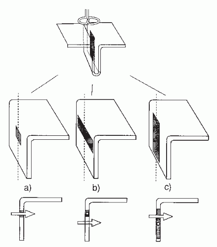 Figure 42.5 Schematic illustration of equivalent current dipole (ECD) locations when the source is (A) a layer of less than 2 cm in diameter, (B) a layer with angular extension, and (C) a layer extended along the radius of the sphere. The activity is assumed to occur in the wall of a cortical fissure. This behavior depends slightly on the coil configuration used. (Adapted from Hari R. On brain’s magnetic responses to sensory stimuli. J Clin Neurophysiol. 1991;8:157-169.) |
When a single current dipole is used to model an extended cortical area consisting of a layer of dipoles, the estimates of dipole depth and, consequently, of dipole strengths may be erroneous (Fig. 42.5). Better source models are thus needed for extended areas. When multiple brain regions are simultaneously active, the relative contribution of each area to the measured signal depends on its site, strength, and synchrony. Multidipole models with time-varying source strengths are useful in interpreting the resulting complex field patterns (47).
NEURAL CURRENTS UNDERLYING THE CURRENT DIPOLE
To understand the cellular events underlying the ECD, it is reasonable to divide the currents associated with postsynaptic potentials (PSPs) to transmembrane currents at the active synaptic area, intracellular currents within the neuron, and extracellular “volume” currents. Transmembrane currents are the driving force for both intra- and extracellular current flow. ECD calculated from the measured MEG signals reflects the direction of the net intracellular current flow. A PSP at the end of one dendrite produces an “elementary” dipole moment Q = Iλ (˜10-14 nAm), where I is the intracellular current driven by the synapse and λ is the length constant of the cell membrane (48). The strength of the observed dipole moment can be strongly affected by the simultaneous calcium currents.
Since it is not known how many PSPs occur synchronously in each pyramidal cell and how much cancellation takes place within the cortex, it is not possible to derive accurate estimates for the source area of a typical evoked response on the basis of cell/synapse density and the size of the elementary dipole. Okada et al. (49) note that many animal species across a wide phylogenetic scale (turtle, guinea pig, and swine) show an apparent invariance in the maximum current dipole moment density of 1 to 2 nAm/mm2. Considerably smaller dipole moment densities have been estimated on the basis of available information on intracortical current densities and values of cortical λ (50). However, intracortical current densities depend strictly on the degree of neuronal synchrony, and thus on the specimen studied, and λ may vary according to background activity (51). Since λ is proportional to the square root of the fiber diameter, the dipole moments weigh the larger neurons.
Glial cells may affect the MEG and EEG signals: they change the return paths of volume currents and have activation latencies that fit with the occurrence of long-latency-evoked responses. Several important electrical events probably remain beyond the reach of both MEG and EEG measurements. For example, intracortical short-distance interactions are—when viewed from the top of the cortex—radially symmetric; only their net effect along the dendrites of the pyramidal cells gives rise to an MEG signal.
MINIMUM-NORM ESTIMATES
An example of a different approach to the neuromagnetic inverse problem is the minimum-norm estimate (MNE) presentation of the source currents (52). MNE gives the most probable current distribution, in the sense of the minimum norm, giving rise to the recorded magnetic field. Calculation of MNE does not require specific assumptions about the source configuration (one dipole, multiple dipoles, quadrupoles, etc.), which is an advantage when there is no basis for explicit models. On the other hand, the unconstrained MNE solution favors superficial currents and does not give a reliable estimate of the source depth. Therefore MNE solutions have been weighted with constraints based on the known brain anatomy and physiology, especially source depth (53,54). Minimum-current estimates (MCEs) (55), a subclass of MNE solutions that give more local solutions, have been applied for visualization and analysis of single-subject and group-level MEG data. One example of MCE visualization is given in Figure 42.6.
The distributed MNE-based source activations often look “more physiologic” than the point-like current dipoles, and therefore current dipoles have been considered old-fashioned and less appropriate than the distributed models to describe the complex brain activity. However, a word of caution has its place
here because the appearance of the result depends strongly on the method used: the MNE approach will give a distributed solution and the dipole approach a local solution, whatever the real current distribution is (see Ref. (16))! In general, both dipole and MCE solutions give rather similar results, although the temporal accuracy may be better with dipole modeling and the group data may be easier to visualize with MCE; however, even well-informed users tend to report more false positives with MCE than with current dipole modeling (56).
here because the appearance of the result depends strongly on the method used: the MNE approach will give a distributed solution and the dipole approach a local solution, whatever the real current distribution is (see Ref. (16))! In general, both dipole and MCE solutions give rather similar results, although the temporal accuracy may be better with dipole modeling and the group data may be easier to visualize with MCE; however, even well-informed users tend to report more false positives with MCE than with current dipole modeling (56).
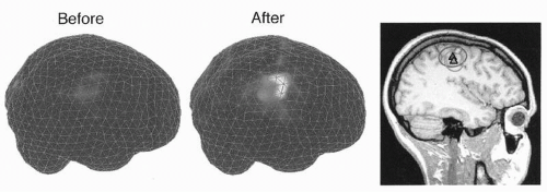 Figure 42.6 Minimum current estimates of the 20-Hz band activity projected to the brain surface of a single subject before (left) and after (middle) oral benzodiazepine administration; the brain is viewed from right. Coregistration of the sources on the subject’s MRI on the right indicates activation of the primary motor cortex, with virtually identical source areas before and after application of benzodiazepines. (Adapted from Jensen O, Goel P, Kopell N, et al. On the human motor-cortex beta rhythm: sources and modelling. Neuroimage. 2005;26:347-355.) |
COMBINATION OF MEG WITH MRI/fMRI/PET DATA
Functional information from MEG is at present routinely combined with structural information from MRI. Moreover, all source estimates could be improved by constraints based on the known anatomy of the brain, derived from MRI data, and forcing the dipoles/currents to the cortical tissue. In preoperative evaluation, reconstruction of the three-dimensional outer surface of the brain from MRI scans helps the surgeon to recognize the landscape after opening the skull when the brain tissue retracts and the relationship between the brain and the landmarks on the skull changes (57). Adding surface vessels to the reconstruction further facilitates the orientation during surgery (58) (Fig. 42.30).
Compared with PET and fMRI (59), the advantage of MEG is its good temporal resolution that allows monitoring of cortical dynamics in millisecond scale. In combined use of multiple methods, active brain regions have been first determined with PET/fMRI and then used as source constrains in the inverse solution of the MEG data to reveal the corresponding temporal behavior. However, not all changes in the synchronization of a neuronal population, reflected in the MEG/EEG signals, induce significant changes in the mean neuronal firing rates or the blood flow and metabolism, and vice versa. Therefore MEG and fMRI results may significantly differ in certain conditions (60), and the MEG/EEG and fMRI/PET methods remain complementary in studies of human brain function. New approaches to combine fMRI and MEG data have been introduced, and the theoretical basis of the fusion is improving (see, e.g., Ref. (61)).
VOLUME CONDUCTOR MODELS
The sphere model works well in most areas of the head when the radius of the sphere is fitted to the local radius of curvature of the measurement area (62), likely because the realistic noise largely masks the errors caused by the different conductor models (63). Realistic head models that take more computing time may be needed for proper modeling of the temporobasal and frontobasal brain areas (64). Fortunately, it is sufficient for MEG to model the intracranial space since only a relatively small proportion of the currents flow in the poorly conducting skull. In contrast, proper modeling of the EEG signals necessitates a multicompartment model consisting of 3 to 4 concentric layers with known resistivities.
Some nonspherical electric inhomogeneities may also affect MEG distributions (65). For example, the falx cerebri may change volume current paths and lead to slight mislocalizations of current dipoles in the mesial wall of the hemisphere. There has been discussion about the significance of holes in the skull to the distribution of volume currents. In the intact human skull, the main holes are in the base of the skull and in the orbits. The absence of electro-oculographic artifacts in intracranial recordings from the frontal lobe (66) suggest a rather good isolation between the outer and the inner sides of the skull. Therefore the effects of normal holes of the skull seem negligible for the interpretation of MEG distributions, as is also supported by calculations showing that radial anisotropy added to a spherically symmetric conductor does not affect the external magnetic field (67).
PRACTICAL ISSUES
Successful clinical MEG recordings need sophisticated instrumentation and close interdisciplinary collaboration. The experimental situation introduces some restrictions. Since the head has to be immobile, recordings cannot be performed during major motor seizures, and problems are encountered in studies of uncooperative subjects who either cannot keep still during the recording or who are not willing or able to perform the tasks. However, continuous monitoring of the head position is currently possible with some neuromagnetometers. Moreover, multichannel MEG mappings are quick to perform and the relative locations of the sensors, required for accurate source analysis, are exactly known without extra effort.
Figure 42.7 illustrates some common MEG artifacts. Since significant contamination can be caused by eyeblinks and movements (68), the electro-oculogram should be used to reject, or at least monitor, contaminated signals. Muscular artifacts cause problems less frequently. Magnetic lung contamination or magnetic material in clothing can cause respiration-related slow shifts. Cardiac artifacts can be either magnetocardiographic signals (69,70), picked up at distance, or ballistocardiographic fluctuations, caused by the movement of magnetized material at the rhythm of the cardiac cycle. For recognition of both artifacts, simultaneously recorded ECG is essential: the magnetocardiogram coincides with the ECG, whereas the main peak of the magnetic ballistocardiogram is broader and lags the QRS complex by several hundred milliseconds.
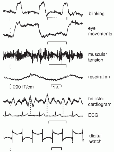 Figure 42.7 Different artifacts in magnetoencephalogram (MEG) recordings of spontaneous brain activity over the temporal area; the measurements were made with a planar gradiometer. Blinking and vertical eye movements produce signals of about equal size; for horizontal eye movements the signals are similar in waveform but have different spatial distributions. Muscular tension refers to biting the teeth together. Respiration artifacts were due to a metallic piece over the chest of the subject. The magnetic ballistocardiogram was due to movement of magnetized metal on the bed, on which the subject was lying on his left side. Note the timing differences between the maximum signals in the electrocardiogram (ECG) and the ballistocardiogram. The lowest artifact was due to a digital watch 70 cm from the Dewar. |
All magnetic materials must be avoided in the clothing of the subject. Although intraoral metallic devices for orthodontics or magnetized material used in staples and sutures during brain surgery may contaminate the MEG measurement, recent development of signal-space separation (SSS) method and its temporal extension (tSSS) help to remove artifacts in the postprocessing phase (71, 72 and 73). It is even possible to clean the MEG data from artifacts elicited by deep brain stimulator (74), as is illustrated in Figure 42.8.
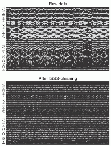 Figure 42.8 The effect of tSSS artifact suppression on spontaneous magnetoencephalogram (MEG) of a person with deep brain stimulator. Top: Spontaneous MEG signals from the left hemisphere when the stimulator was on. The approximate locations of the planar gradiometers are indicated; total duration 30 seconds. Bottom: After tSSS when even the normal posterior alpha activity is visible. The amplitude scales are the same in both panels. Courtesy of Jyrki Mäkelä, Helsinki University Central Hospital. (See color insert) |
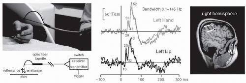 Figure 42.9 Tactile stimulator made of a bundle of optical fibers and the somatosensory responses obtained by stimulating the left hand and the left lip. The corresponding source areas in the right-hemisphere primary somatosensory cortex and the current directions are indicated on the right (hand up, lip below). (Adapted from Jousmäki V, Nishitani N, Hari R. Brush stimulator for functional brain imaging. Clin Neurophysiol. 2007;118:2620-2624.) (See color insert) |
Special attention must also be paid to the proper design of stimulators. High-quality sounds can be produced with electroacoustic transformers placed outside the shielded room and connected through plastic tubes to the subject; the system may need sophisticated equalizing to guarantee flat frequency transfer. Excessive artifacts from electric somatosensory stimuli can be avoided by twisting the stimulator wires tightly together. Multichannel devices with balloon diaphragms driven by compressed air (75) provide a nice and artifact-free method for tactile stimulation. A hand-held bundle of optical fibers, half emitting red light and the other half detecting the reflected light from the skin can be used to evoke reliable somatosensory responses to taps to the skin (76); see Figure 42.9.
Noxious laser heat stimuli for pain studies can be brought to the shielded room via optical cables. Visual stimuli can be transmitted through mirrors, a data projector, a bundle of optic fibers, or the subject can view a monitor through a hole in the wall. EEG can be measured with nonmagnetic electrodes and wires without causing problems to the MEG recordings. Eye tracking can be performed during the MEG recordings with an infrared camera.
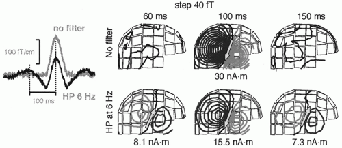 Figure 42.10 Dangers of filtering, illustrated with simulated data. A current dipole with a monophasic activation curve (gray line on the left, “no filter”) and with 30 nAm dipole moment was inserted to a site corresponding to the right auditory cortex. The field patterns above show a dipolar field pattern at peak activation at 100 msec. After high-pass filtering at 6 Hz the waveform changes (black curve on the left, “HP 6 Hz”) and ghost sources appear at 60 and 150 msec. |
Figure 42.10 draws attention to dangers of filtering. A too high high-pass filter setting will cause well-known distortions in the signal waveforms but—what may be less obvious—also transfer the dipolar field patterns, with opposite polarities, to latencies distant from the real signal and thereby lead to erroneous interpretations of brain activation.
ANALYSIS OF SPONTANEOUS ACTIVITY
Very useful information about spontaneous activity (for a review, see Ref. (11)) can be obtained by calculating frequency spectra of the signals (Fig. 42.11) and by mapping the abundance of different frequencies at various sensor sites. The sources can then be identified either in time or in frequency domain (77, 78 and 79). In multichannel recordings, cross-spectra between channels suggest which signals arise from the same source, and time lags may tell about the sequence of activation.
One may quantify the level of different brain rhythms by using time-frequency representations, or more simply using the temporal spectral evolution (TSE) method (80) by focusing on one frequency band at a time. The TSE method resembles the
“event-related desynchronization” technique (81) used to study task-dependent changes in the human scalp EEG. However, TSE preserves the original units and the signal levels can thus be directly compared with the sizes of evoked responses. In TSE, the brain signals are first bandpass filtered, then rectified (taking absolute values of the signals), and thereafter averaged with respect to the triggering event. Thus, all signals that are time-locked but not exactly phase-locked to the event will be detected.
“event-related desynchronization” technique (81) used to study task-dependent changes in the human scalp EEG. However, TSE preserves the original units and the signal levels can thus be directly compared with the sizes of evoked responses. In TSE, the brain signals are first bandpass filtered, then rectified (taking absolute values of the signals), and thereafter averaged with respect to the triggering event. Thus, all signals that are time-locked but not exactly phase-locked to the event will be detected.
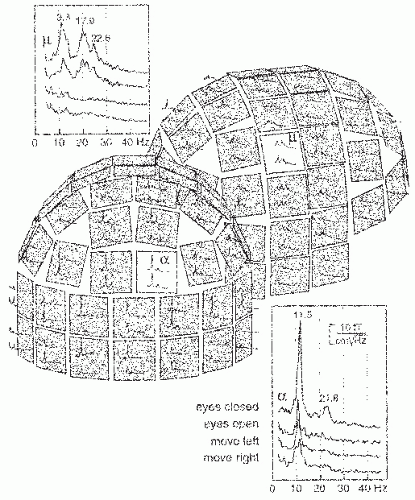 Figure 42.11 Amplitude spectra from a 1-minute period of spontaneous activity when the subject was resting with eyes closed. Two orthogonal derivatives of the radial magnetic field were measured at each location, along the longitude and latitude. The insets show reactivity of the α- and µ-rhythms to opening of the eyes and to movements of the left and right hand. (Adapted from Salmelin R, Hari R. Characterization of spontaneous magnetoencephalogram (MEG) rhythms in healthy adults. Electroenceph Clin Neurophysiol. 1994;91:237-248.) |
Sometimes one may be interested in just seeing the signal waveform and the temporal changes in the field pattern. This type of analysis, which resembles the classical use of EEG recordings, can be helpful in screening candidates for surgical treatment: clear changes of the field pattern from one irritative phenomenon to the next discourage the assumption of a local onset of the discharge, although they do not rule out a deeper common trigger.
Due to noise problems and the use of single-channel instruments, the first studies of epileptic MEG activity employed averaging, with the simultaneously recorded EEG signal as a trigger (32,82). The drawback of such a procedure is that the choice of the trigger channel largely determines the observed activity, and the method works only if well-discernible spikes or sharp waves are present. With multichannel low-noise instruments, averaging is necessary only for the detection of prespikes, which might be accurate indicators of the onset area of the paroxysmal activity (83). With template matching, signals can be automatically classified and the source locations determined separately for each class.
SPONTANEOUS ACTIVITY OF AWAKE NORMAL SUBJECTS
Alpha Rhythm from Parieto-Occipital Areas
The typical parieto-occipital alpha rhythm, with a peak frequency around 10 Hz, is damped by opening the eyes (Fig. 42.11). In the first study of the human magnetic alpha rhythm (1), a phase reversal was observed between signals measured from the right and left hemispheres, and the currents were therefore suggested to be parallel to the longitudinal fissure.
Later, the sources of the alpha rhythm have been suggested to cluster mainly in the region of the calcarine sulcus (84) and around the parieto-occipital sulcus (POS) (85, 86, 87 and 88). Figure 42.12, based on whole-scalp MEG recordings, shows sources in both of these locations, typically the POS region is the far most dominant source of the MEG alpha rhythm.
Vvedensky et al. (85) suggested that alpha spindles often have the same generators for about 1 second, whereas the sources differ for successive spindles. Later, a multitude of MEG alpha sources were found with the help of “signal-space analysis” (89). Different spindles seemed to have different sources but the source configuration of one spindle was rather stable. Later recordings, analyzed with time-varying fixed-location dipole models, however, suggest that a typical alpha spindle cannot be explained by a single source (88).
The parieto-occipital alpha rhythm is strongly suppressed during visual stimuli, visual memory tasks, and visual imagery (90, 91, 92 and 93). When the subject has to differentiate between visually presented images of objects vs. nonobjects, the poststimulus alpha level is consistently higher after nonobjects (94). This
modulation may reflect interaction between the dorsal and ventral visual pathways during an attention-demanding task. The level of parietal alpha activity has been related to memory load (95).
modulation may reflect interaction between the dorsal and ventral visual pathways during an attention-demanding task. The level of parietal alpha activity has been related to memory load (95).
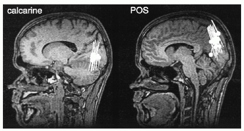 Figure 42.12 Sources of alpha oscillations superimposed on two sagittal MRI slices demonstrating a calcarine (left) and a parieto-occipital (right) source cluster. Source current orientations are also indicated. (Adapted from Hari R, Salmelin R, Mäkelä JP, et al. Magnetoencephalographic cortical rhythms. Int J Psychophysiol. 1997;26:51-62.) |
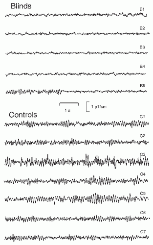 Figure 42.13 Traces of parieto-occipital alpha activity from five early blind subjects and seven control subjects. The blind subjects were 25 to 32 years in age. Subjects B2 and B3 were able to see some light; subject B5 is blind due to retinal cancer and has seen light only during her first year. M. Huotilainen and T. Kujala participated in data collection. |
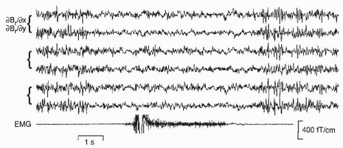 Figure 42.14 Spontaneous magnetic activity over the rolandic area, shown on six gradiometer channels, when the subject has his eyes open and clenches his contralateral fist (see the electromyogram [EMG] channel). (Unpublished data from F. Lado and R. Hari.) |
Early visual deprivation may lead to the abolishment of parieto-occipital spontaneous rhythms: from the five early blind subjects in Figure 42.13, four do not display alpha activity and opening/closing the eyes did not have any effect on their brain rhythms. Only one subject (B5) has rhythmic alpha-like activity; she had lost her sight earlier than the other four subjects. The reason for the observed alpha absence in blinds, also known from EEG recordings (96), is unknown, but it certainly speaks against a purely idling nature of the normal alpha rhythm; otherwise one might expect strong alpha during the continuous lack of visual input.
Mu Rhythm from Sensorimotor Areas
The electroencephalographic µ-rhythm has a magnetic counterpart that starts to dampen 1 to 2 seconds before a movement (Fig. 42.14). In association with unilateral movements, the suppression is bilateral, although contralaterally dominant (97).
The µ-rhythm consists of two main frequency components, one around 10 Hz and the other around 20 Hz (see inset in Fig. 42.11); however, these two frequencies are usually not exact harmonics and show independent temporal behaviors (98). Additional evidence for functionally separate frequency components of the µ-rhythm derives from the source locations, which center on average 5 mm more anterior for the 20 Hz than the 10 Hz frequencies (80), suggesting the existence of separate precentral (20 Hz) and a postcentral (10 Hz) rhythms (Fig. 42.15).
In addition to movements (99), the magnetic µ-rhythm is modified by electric stimulation of peripheral nerves, with a more clear increase, “rebound” of the 20-Hz than the 10-Hz component around 400 msec after the stimulus (80,97). The poststimulus rebound is abolished when the subject moves the fingers of the same hand. Interestingly, a similar, but weaker,
suppression is seen when the subject just imagines making the movements, indicating involvement of the primary motor cortex in motor imagery (100). Suppression of the rebound, as a sign of motor-cortex activation, also occurs when the subject just views another person to make certain movements (Fig. 42.16) (101).
suppression is seen when the subject just imagines making the movements, indicating involvement of the primary motor cortex in motor imagery (100). Suppression of the rebound, as a sign of motor-cortex activation, also occurs when the subject just views another person to make certain movements (Fig. 42.16) (101).
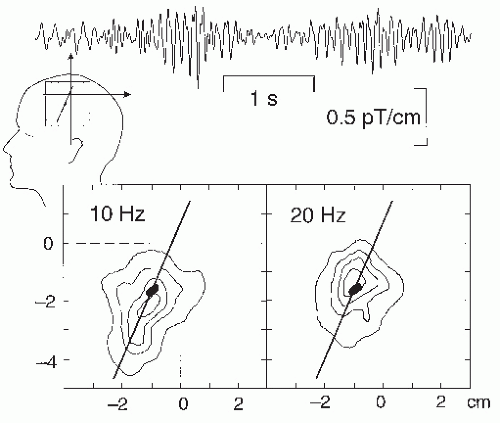 Figure 42.15 Top: A 5-second trace of magnetic µ-rhythm from the rolandic region. Bottom: Isodensity clusters of sources of 10- and 20-Hz oscillations over the rolandic region of one subject, based on thousands of equivalent current dipole (ECD) locations. The black ovals show the area activated by median nerve stimulation at the wrist, and the line shows the estimated course of the rolandic fissure. (Adapted from Salmelin R, Hari R. Spatiotemporal characteristics of rhythmic neuromagnetic activity related to thumb movement. Neuroscience. 1994;60:537-550.) |
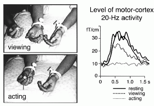 Figure 42.16 Level of the 20-Hz rolandic activity after stimulation of the contralateral median nerve when the subject either rested (solid lines), viewed another person to manipulate a small object with the right hand fingers (dashed line; “viewing”), or manipulated the same object herself (“acting”). The sources of these 20-Hz signals were in the precentral primary motor cortex. (Adapted from Hari R, Forss N, Avikainen S, et al. Activation of human primary motor cortex during action observation: a neuromagnetic study. Proc Natl Acad Sci USA. 1998;95:15061-15065.) |
The 20-Hz rebounds do—whereas the 10-Hz rebounds do not—follow the moved body part in a somatotopic manner: they appear at lateral rolandic areas after mouth movements, more medially after finger movements, and close to midline after foot movements (102).
Recent MEG recordings after oral administration of benzodiazepine demonstrated a strong increase in the power of approximately 20-Hz oscillations in both hemispheres, with sources in the primary motor cortex close to the hand area (103) (Fig. 42.6). These data suggest that the motor cortex is an important effector site of benzodiazepine, and they also agree with the proposed generation of the rolandic 20-Hz oscillations in the motor cortex. The frontal-lobe dominance of benzodiazepine-related scalp-EEG beta activity can be explained by tangential current dipoles in the wall of the central sulcus.
Oscillatory Cortex-Muscle Coupling
The human rolandic MEG activity has been observed to have a close temporal relationship to peripheral muscular activity (54,104, 105 and 106). For example, during isometric contraction of different muscles, the muscular and cortical signals are coherent at frequencies varying between 15 and 33 Hz in individual subjects (106). The sites of maximum coherence in the motor cortex show gross somatotopic organization, with activations during foot muscle contraction closer to the head midline than during hand muscle contractions (Fig. 42.17).
The MEG signals lead the EMG signals in time, with increasing time lags with increasing brain-muscle distance. Such data strongly suggest that the 20-Hz rolandic rhythm reflects, at the population level, the common central drive to spinal motoneurons (for reviews, see Refs. (107,108)). The corresponding cortex-muscle coherence can also be shown with EEG recordings (109).
The MEG signals lead the EMG signals in time, with increasing time lags with increasing brain-muscle distance. Such data strongly suggest that the 20-Hz rolandic rhythm reflects, at the population level, the common central drive to spinal motoneurons (for reviews, see Refs. (107,108)). The corresponding cortex-muscle coherence can also be shown with EEG recordings (109).
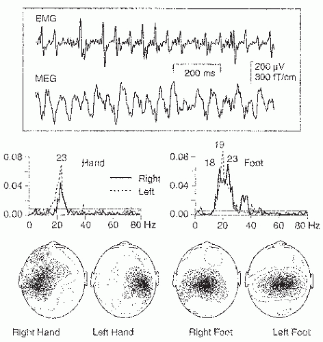 Figure 42.17 Top: Surface electromyogram (EMG) from isometrically contracted left hallucis brevis muscle and simultaneously recorded magnetoencephalogram (MEG) signal over the parietal midline (3 to 100 Hz). Middle: Coherence spectra between MEG and EMG during isometric contraction of small hand and foot muscles (left- and right-sided contractions superimposed). Bottom: Spatial distributions of the strongest peaks of the coherence spectra. (Adapted from Salenius S, Portin K, Kajola M, et al. Cortical control of human motoneuron firing during isometric contraction. J Neurophysiol. 1997;77:3401-3405.) |
Studies with different gripping tasks have led to the proposal that the cortical oscillations have a role in recalibrating the control system after a change in the cortex-muscle relationship (110,111). At strong contractions, the frequency of the coherence jumps from 20 to 40 Hz (“Piper rhythm”; (112,113)). The cortex-muscle coherence provides a complementary tool to identify the primary motor cortex as a part of preoperative functional mapping (58).
Gross et al. (114) demonstrated, using a sophisticated dynamic imaging of coherent sources (DICS) method, developed to characterize synchronously firing neural networks in different parts of the brain, that 6- to 9-Hz velocity changes of slow finger movements are directly correlated to oscillatory activity of the primary motor cortex. Moreover, the coherence patterns suggested that the pulsatile velocity changes were sustained by a cerebellar drive through thalamus and premotor cortex.
Tau Rhythm from Auditory Areas
A third MEG rhythm, which I have started to call τ-rhythm (τ referring to temporal lobe), was described by Tiihonen et al. (115). This 8- to 10-Hz oscillatory activity is best seen in the planar gradiometer recordings just over the auditory cortex. Occasionally the rhythm is reduced by sound stimuli, such as bursts of noise, but it is not dampened by opening the eyes—a feature clearly distinct from the occipital alpha. The sources of single-tau oscillations cluster to the supratemporal auditory cortex close to the generations site of auditory-evoked fields, with right-hemisphere dominance (Fig. 42.18) (116).
On the basis of the observed current orientations, the corresponding electric τ-rhythm should be seen mostly in the frontocentral midline where the tau sources, with dipole moments of 40 nAm, would lead to potentials of about 10 to 20 |V. In fact, such an EEG rhythm may appear during drowsiness: Decreased vigilance is often considered to be associated with a “spread” of occipital EEG alpha toward more anterior regions, with simultaneously slightly decreasing frequency (117,118). A real spread of the alpha would be in clear contrast to the fixed, although distributed, generators of alpha activity, and a more plausible explanation is that the anterior “alpha” in fact reflects “tau” generated in the supratemporal auditory cortex.
The combined MEG and EEG data of Lu et al. (119) would agree with such a hypothesis: During the awake state (the first panel of Fig. 42.19) the occipital EEG displays rhythmic 10 to 11 Hz alpha activity, and the simultaneous MEG in the temporal region is of low amplitude, with little rhythmic activity. However, when the occipital electric alpha becomes discontinuous during light drowsiness (Stage 1a) and seems to spread more anteriorly, with slightly slowed down frequency, rhythmic activity of the same frequency appears in the MEG sensors over the temporal lobe.
Therefore, the apparent spread of the EEG “alpha” during drowsiness might reflect changed relative contributions from the occipital alpha and from the temporal tau generators. Epidural electrode recordings (120,121) show that also the temporal-lobe 6- to 11-Hz activity arising from the convexial cortex is strikingly resilient to decreased vigilance.
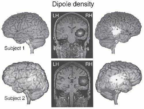 Figure 42.18 Locations of equivalent current dipoles for the tau oscillations (6.5 to 9.5 Hz range) in two subjects. The sources (clusters of white dots) are projected to the surface of the brain and shown on the subject’s own MRI. The black dot indicates the source of the auditory N100m response. In the coronal sections in the middle, the dipole distributions are presented as contour plots, with highest dipole densities in white and lowest in black. (Adapted from Lehtelä L, Salmelin R, Hari R. Evidence for reactive magnetic 10-Hz rhythm in the human auditory cortex. Neurosci Lett. 1997;222:111-114.) |
A Note on Nomenclature
The existence of local cortical rhythms explains in part the confusion in the literature concerning effects of various tasks on the spontaneous EEG. Some people consider alpha to refer to the occipital “Berger rhythm,” independently of its shape (i.e., frequency composition), whereas others refer to alpha as all signals falling in the 8- to 13-Hz frequency range, independently of the brain area where they are generated. To avoid confusion, it would be necessary to characterize each rhythm both by its site of origin and by its frequency range.
Other Brain Rhythms
A 7- to 9-Hz “sigma” rhythm has been demonstrated in MEG recordings in the second somatosensory cortex (122). Single median-nerve stimuli elicited some sigma oscillations, and the level of sigma was enhanced during rhythmic stimulation at the rhythm’s dominant frequency.
Theta-range MEG activity has been scarcely studied. Sasaki et al. (123) recorded 5- to 7-Hz MEG signals from the frontal cortex during mental calculation and intensive thinking. Tesche (30) estimated the temporal waveforms of sources (computationally) inserted to the hippocampus and found in some subjects around 5-Hz rhythmic activity during mental calculation.
Since 1980s, much attention has been paid to the 40-Hz frequency band, often supposed to have a role in perceptual binding
(124,125). Both stimulus-related and later “induced” 40-Hz activity has been reported, with differences between visual EEG and MEG 40-Hz signals (53,126). Even higher MEG frequencies (from 30 to 150 Hz) have been recently used to demonstrate dissociation between visual awareness and spatial attention (127). Although the 40-Hz activity, according to animal experiments, results from thalamocortical interaction, it is at present unknown how strongly the subcortical structures contribute to the MEG signals that are biased toward cortical currents.
(124,125). Both stimulus-related and later “induced” 40-Hz activity has been reported, with differences between visual EEG and MEG 40-Hz signals (53,126). Even higher MEG frequencies (from 30 to 150 Hz) have been recently used to demonstrate dissociation between visual awareness and spatial attention (127). Although the 40-Hz activity, according to animal experiments, results from thalamocortical interaction, it is at present unknown how strongly the subcortical structures contribute to the MEG signals that are biased toward cortical currents.
Related posts:

Stay updated, free articles. Join our Telegram channel

Full access? Get Clinical Tree


