Computer-Assisted EEG Pattern Recognition and Diagnostic Systems
Fernando H. Lopes Da Silva
If someone would compare older editions of this chapter with the present one, he or she would notice how the field of computerized diagnostic systems has rapidly evolved in the last decade that is reflected in the emergence of new algorithms every year, while some older ones have become obsolete. Nonetheless, much of the older literature continues to be valid inasmuch as it illustrates basic concepts and may guide new researchers to find their way in this frontier between clinical neurophysiology and the technology of applied signal analysis. This kind of review of relatively old literature may help to avoid each generation trying to invent the wheel again. Here we pay attention also to recent developments and new trends. We should note that some new algorithms are simple variants of previous approaches. Very often the performance of the new ones is not assessed with respect to the older versions that leads to some lack of transparency in this field.
A common denominator of the field of computer-assisted EEG diagnostic systems is the application of pattern recognition methods. The latter constitute a general class of procedures applicable in a variety of scientific areas. The first operation in EEG analysis is to define a pattern, that is, to choose a set of features that are potentially important in identifying the phenomena of interest. This set of features constitutes a pattern. The second operation may be the classification or clustering of the set of features. According to the former one must assume a priori that there exists a number of classes (e.g., clinical normal/abnormal) to which the objects must be allocated; according to the clustering approach, however, it is not necessary to define a predetermined number of classes. Rather, in this case the aim is to find clusters of objects based on a given statistical criterion. In the classification approach one chooses a group of EEGs, the so-called learning set, to determine the set of features that gives the best possible discrimination between the classes, for example, applying Fisher’s linear discriminant analysis. Thereafter, the best set of features can be used to classify any other group of EEGs that constitute the test sets.
Clustering requires little or no specific a priori knowledge; the objects are grouped in clusters applying a clustering algorithm. The user must determine, however, the most convenient level at which clustering must be stopped, according to the specific problem being analyzed. Thereafter, the relevance of the clusters obtained with respect to the specific clinical application, or any other application of interest, must be evaluated.
Since in EEG analysis, most methods of analysis follow a pattern recognition approach, explicitly or not, we consider here the most important aspects of such an approach in relation to general problems of automatic EEG diagnosis. For a thorough treatment of pattern recognition theories, the reader is referred to the classic books of Duda and Hart (1), Mendel and Fu (2), and Tou and Gonzalez (3), and to the review of Demartini and Vincent-Carrefour (4) that deals with the specific field of EEG.
FEATURE EXTRACTION: SPECIFIC PROBLEMS
The usefulness of any EEG analysis method depends, to a large extent, on the choice of the set of features that is relevant to answer the question being investigated. In this section we consider, first, the main types of features used in EEG analysis in general terms; then we examine how these features can be incorporated into EEG classification systems in specialized cases.
Time-Domain Analysis Methods
Methods aiming at extracting time-domain EEG features were used in the early period of EEG quantification but are less used recently. The main features used in this context are derived from EEG amplitude analysis: the features ordinarily chosen are mean (m), standard deviation (σ), skewness, kurtosis, and coefficient of variation [(σ/m) × 100] of EEG signals; these are computed from the original signal as discussed in Chapter 54. Furthermore, one can also define similar features for the rectified signal: mean, standard deviation, and coefficient of variation. Furthermore, interval analysis of EEG signals yields a number of other features: average frequency of zero crossings of the original signal and also of its first and second derivatives. The combination of amplitude and interval analysis (see Chapter 54) yields a set of features that can characterize EEG signals; in addition to those described above, a few others may be chosen such as the signal half-wave length and its derivatives (mean, standard deviation, and range), peak-to-peak values per wave (mean and standard deviation), and amplitude range (i.e., the difference between the largest and the smallest amplitude value within a certain time epoch). Other features that have been included in this kind of analyses are Hjorths parameters: activity, mobility, and complexity, and parameters extracted using time-frequency analyses, for example, those obtained by wavelet decomposition, as explained in Chapter 54.
Spectral Analysis Using Nonparametric Methods
The most common features extracted from EEG, however, are derived by way of spectral analysis, such as the spectral intensity within the classic frequency bands, namely the mean spectral intensity (power or amplitude) and the average frequency. Although this may be rather trivial, it is important to consider the fundamental question of how to define the EEG frequency bands. According to the generally accepted empirical definitions, one may use the subdivision indicated in Table 56.1. A question that should be asked is whether the activities in different frequency bands are independent, or not. This question can be answered by means of multivariate statistical analysis of EEG spectral values. This issue has been investigated thoroughly in the 1970s when the first computerized systems were started to be developed. Hermann et al. (7) using factor analysis chose 57 relative power values in frequency bands between 1.5 and 30 Hz with frequency resolution f = 0.5 Hz, as well as absolute power values. In this way, it was found that the power spectrum could be broken down into the frequency bands indicated in Table 56.1. Dymond et al. (8) also performed factor analysis of power spectra (log transformed) of bilateral centro-occipital leads and extracted four main factors having high loadings within the following frequency bands: 0 to 8, 6 to 12, 12 to 20, and 20 to 30 Hz; they also extracted factors associated with EEG asymmetry.
Table 56.1 EEG Features Obtained from Spectral Analysis | ||||||||||||||||||||||||||||||||||||||||||||||||||||||||||||||||||||||||||||||||||||||||||||||||||
|---|---|---|---|---|---|---|---|---|---|---|---|---|---|---|---|---|---|---|---|---|---|---|---|---|---|---|---|---|---|---|---|---|---|---|---|---|---|---|---|---|---|---|---|---|---|---|---|---|---|---|---|---|---|---|---|---|---|---|---|---|---|---|---|---|---|---|---|---|---|---|---|---|---|---|---|---|---|---|---|---|---|---|---|---|---|---|---|---|---|---|---|---|---|---|---|---|---|---|
| ||||||||||||||||||||||||||||||||||||||||||||||||||||||||||||||||||||||||||||||||||||||||||||||||||

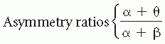
It should be noted, however, that applying factor analysis to sets of power spectra is not simple. The results depend on (i) whether the spectra are expressed in power or in root mean square (RMS) values, (ii) the way the spectra have been normalized, (iii) the derivations that were included, and (iv) the subject population. The results of an investigation of the University Hospital of Utrecht (Wieneke, personal communication), which factorized frequency bands of power spectra (logarithmic values) obtained from eight symmetrical derivations in 89 patients, are shown in Table 56.1; in this case, normalization was performed using the band from 5 to 20 Hz as reference. The distribution of the most important frequency factor loadings obtained in this way for different derivations is given in Figure 56.1. We should emphasize that this type of analysis is sensitive to normalization and scaling. It is remarkable, however, that the different methods presented in Table 56.1 yield results that display a considerable degree of overlapping with respect to the different frequency bands. The frequency bands calculated in this way are also clearly compatible with those used in classical EEG; therefore, it may be said that a subdivision in frequency bands as used by Matousek and Petersén (5) or Gotman et al. (9) is acceptable for routine clinical EEG analysis. If one deals with a completely defined group of EEGs (e.g., in psychopharmacologic studies where one has a group of subjects receiving a drug and a control group), factor analysis may preferably be applied to such a specific group in order to define the optimal frequency bands that should be used in that specific study. Within the defined frequency bands, several primary spectral features, such as absolute power intensity in µV2 or in dB, relative power, square root of power, and average
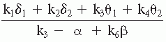
frequency within a band, can be computed. Secondary spectral features can also be derived. Several types of secondary features have been proposed based on empirical criteria; clinical application has validated those proposed by Matousek and Petersén (5) and by Gotman et al. (9). Matousek and Petersén (5) investigated 20 features extracted from the frequency spectrum of each EEG derivation. This study was based on the authors’ claim that an increased amount of slow frequency in the EEG in abnormal cases might be considered analogous to the relatively large amount of slow activity seen in the normal but immature EEG. Initially, the EEG score chosen as being the most clearly age-related was the ratio between theta-band activity (3.5 to 7.5 Hz) and the alpha-band activity (7.5 to 12.5 Hz) added with a constant factor.
frequency within a band, can be computed. Secondary spectral features can also be derived. Several types of secondary features have been proposed based on empirical criteria; clinical application has validated those proposed by Matousek and Petersén (5) and by Gotman et al. (9). Matousek and Petersén (5) investigated 20 features extracted from the frequency spectrum of each EEG derivation. This study was based on the authors’ claim that an increased amount of slow frequency in the EEG in abnormal cases might be considered analogous to the relatively large amount of slow activity seen in the normal but immature EEG. Initially, the EEG score chosen as being the most clearly age-related was the ratio between theta-band activity (3.5 to 7.5 Hz) and the alpha-band activity (7.5 to 12.5 Hz) added with a constant factor.
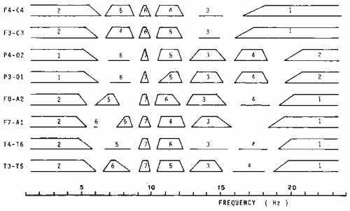 Figure 56.1 Factors found using factor analysis of EEG power spectra. Factor analysis of logarithmic power spectra for several derivations was done; power spectra were normalized in relation to the power within the frequency band between 5 and 20 Hz. Each factor is represented either by a parallelogram or simply by a horizontal line. The latter or the base of the parallelogram indicates the frequency interval within which the factor accounts for more than 50% of the variance; the top line of the parallelogram indicates the frequency interval within which more than 70% of the variance is accounted for by the corresponding factor. The factors are numbered in the order of decreasing eigenvalues from 1 to 6 or 7. A varimax rotation was used. The data were obtained from EEGs of 243 patients, each consisting of 100-second epochs recorded with eyes closed. (Courtesy of G. Wieneke.) |
The same group later reinvestigated this problem (10). They used as normative data the RMS of the spectral values computed within the frequency bands, indicated in Table 56.1, for a number of derivations (FT-T3, C3-C0, T3-T5, P3-01, and the symmetrical ones) of 562 EEG recordings from healthy individuals aged 1 to 21 years. A number of ratios between RMS values were also computed. In total, 20 spectral features per derivation were calculated, as follows: x(1) = delta activity, x(2) = theta, x(3) = alpha 1, x(4) = alpha 2, x(5) = beta 1, x(6) = beta 2, x(9) = alpha 1/alpha 2, x(10) = beta l/(alpha 1 + alpha 2), x(11) = beta 2/(alpha 1 + alpha 2), x(12) = beta 1/beta 2, x(13) = delta/theta, and x(14) = sum of delta, theta, alpha 1, alpha 2, beta 1, and beta 2; features from 15 through 20 are normalized amplitudes in relation to x(14) for the following bands: x(15) = normalized delta, x(16) = normalized theta, x(17) = normalized alpha 1, x(18) = normalized alpha 2, x(19) = normalized beta 1, and x(20) = normalized beta 2.
Friberg et al.’s (10) model is defined by the following linear equation: calculated EEG age = a(0) + a(1)x(1) + … + a(20)x(20). The coefficients a(i), with i = 0 to 20, were estimated by minimizing the sum of squares of the differences between the subject’s actual age and the calculated EEG age. The correlation coefficients between actual and calculated EEG age varied between 0.88 for derivations C3-C0 and C0-C4 and 0.86 for derivations F7-T3 and F8-T4. Those authors found that, according to their model, the calculated EEG age tended to be greater than zero when the line was extrapolated down to an actual age of zero. To avoid this, they introduced two new variables: the calculated EEG maturity and the actual EEG maturity; the former is linearly related to the calculated EEG age and the latter to the actual age. The ratio between calculated and actual EEG maturity is called the ratio of EEG normality, because the authors found that this ratio is closely related to the degree of EEG (ab)normality. To calculate such a ratio, the maximal actual EEG maturity of any individual is fixed to correspond to 22 years (age-related EEG changes are considered to be small beyond that age). The clinical implications of this form of feature extraction and data reduction are discussed below.
Gotman and his collaborators based their procedure for extracting spectral features on the widely accepted assumption that some kind of relation between slow and fast EEG activity should characterize the degree of EEG abnormality. Moreover, they pointed out that a relative measure of spectral intensity is preferable to an absolute measure because the latter depends on
a number of spurious factors (e.g., skull thickness). Therefore, these investigators analyzed the potential of several ratios, for example, (delta + theta)/(alpha + beta), using different weighing factors and frequency band subdivisions, to discriminate the EEG between normal and abnormal subjects (slow-wave type of abnormality). The best weighing factors for different frequency bands and areas are given in Table 56.1. The same investigators introduced still another important spectral feature, a degree of asymmetry. To compute this feature, the scalp was subdivided into four symmetrical regions: frontal (Fp1-F3, Fp1-F7, Fp2-F4, Fp2-F8), temporal (F7-T3, T3-T5, F8-T4, T4-T6), central (F3-C3, C3-P3, F4-C4, C4-P4), and occipital (P3-01, T5-01, P4-02, T6-02). For each region, two asymmetry coefficients were calculated, one for the slow frequencies (weighted delta and theta values as given in Table 56.1) and one for the higher frequencies (weighted alpha and beta values). The value corresponding with the most active hemisphere was always placed in the numerator. Gotman et al. (9) called the display of these ratios extracted from spectral values canonograms (canon is Greek for “ratio”) (Fig. 56.2); the clinical validation of these features is discussed later in this chapter.
a number of spurious factors (e.g., skull thickness). Therefore, these investigators analyzed the potential of several ratios, for example, (delta + theta)/(alpha + beta), using different weighing factors and frequency band subdivisions, to discriminate the EEG between normal and abnormal subjects (slow-wave type of abnormality). The best weighing factors for different frequency bands and areas are given in Table 56.1. The same investigators introduced still another important spectral feature, a degree of asymmetry. To compute this feature, the scalp was subdivided into four symmetrical regions: frontal (Fp1-F3, Fp1-F7, Fp2-F4, Fp2-F8), temporal (F7-T3, T3-T5, F8-T4, T4-T6), central (F3-C3, C3-P3, F4-C4, C4-P4), and occipital (P3-01, T5-01, P4-02, T6-02). For each region, two asymmetry coefficients were calculated, one for the slow frequencies (weighted delta and theta values as given in Table 56.1) and one for the higher frequencies (weighted alpha and beta values). The value corresponding with the most active hemisphere was always placed in the numerator. Gotman et al. (9) called the display of these ratios extracted from spectral values canonograms (canon is Greek for “ratio”) (Fig. 56.2); the clinical validation of these features is discussed later in this chapter.
Other spectral features of interest are the spectral peak frequencies and corresponding bandwidths. There are several algorithms used to calculate peak frequencies: these involve computing a local maximum of the curve defining the spectral density. A peak is said to exist when it rises significantly above its surroundings. The bandwidth is usually calculated as the frequency interval between the 3-dB points at both sides of the peak.
A comprehensive analysis methodology that combines quantitative EEG and EP features is the approach introduced by John and collaborators and reviewed extensively in John et al. (11,12) and Prichep and John (13), under the name of neurometrics. This approach is based on the use of standardized data acquisition techniques, computerized feature extraction, statistical transformations in order to achieve approximately Gaussian distributions, age regression equations, and multivariate statistical methods, namely discriminant and cluster analyses to achieve differential diagnosis between patients’ (sub)populations. In this way, neurometric test batteries were constructed and applied to several clinical problems. A general battery consists typically of the following features: spectral composition, coherence, and symmetry indices of the spontaneous resting EEG; in addition, brainstem auditory evoked potential (BAEP) and brainstem somatosensory evoked potential (BSEP) to unilateral stimuli, checkerboard pattern reversal or flash visual EPs, and cortical EPs to different modalities both to predictable and unpredictable stimuli, are also included. This approach can be implemented in a personal computer.
 Figure 56.2 Canonogram from subject with multiple metastases in right hemisphere. The size of each polygon is proportional to a slow/fast EEG activity ratio, indicator of abnormality for a channel. They are arranged in a topographical pattern corresponding to the position of the derivations on the subject’s head: frontal on top and occipital on bottom. Arrows under horizontal lines indicate the asymmetry in slow EEG activity; arrows above indicate the asymmetry in fast EEG activity. Sixteen channels, anteroposterior bipolar montage covering parasagittal and temporal regions; EEG epoch, 40 seconds. (Adapted from Gotman J. Problems of presentation of analytical results. Electroencephalogr Clin Neurophysiol Suppl. 1978;34:191-197.) |
Profiles of neurometric features that deviate from agematched normal subjects have been obtained in several categories of patients suffering from cognitive disorders (e.g., dementias), psychiatric illnesses (e.g., different types of depressions and of schizophrenia), and neurologic dysfunctions, for example, compromised cerebral blood flow (14), as discussed by John et al. (12) and Prichep et al. (15). The clinical relevance of neurometrics is controversial and has led to publications presenting opposite points of view by John (16) and Fisch and Pedley (17). A special effort was made by John and collaborators to apply the neurometrics approach of quantitative EEG analysis to distinguish subgroups of patients with psychiatric disorders also with the aim of identifying potential responders to pharmacologic treatments (18). This was applied to patients suffering from obsessive-compulsive disorder (OCD) who received treatment with selective serotonin reuptake inhibitors (SSRIs) with the interesting result that the responders and nonresponders presented distinct neurometric profiles (19,20).
Spectral Analysis Using Parametric Methods
In Chapter 54 we discussed the general theory of spectral analysis employing ARMA or AR models. One of the main advantages of these parametric methods of computing power spectra, as proposed initially by Zetterberg (21), is precisely the fact that the use of spectral parameter analysis (SPA) avoids having to subdivide the spectrum in distinct frequency bands
beforehand. The SPA method describes the EEG as resulting from noise sources passed through a set of parallel first- or second-order filters, as illustrated in Figure 56.3. As demonstrated by Isaksson and Wennberg (22), the relevant spectral features can be derived simply. The first-order filter describing the low-frequency band is characterized by two features: the total power G and the total bandwidth (interval from zero to the frequency corresponding to the 3-dB point); each of the second-order filters describing theta, alpha, and beta components is characterized by the three features: G (power), σ (bandwidth), and f (resonance frequency).
beforehand. The SPA method describes the EEG as resulting from noise sources passed through a set of parallel first- or second-order filters, as illustrated in Figure 56.3. As demonstrated by Isaksson and Wennberg (22), the relevant spectral features can be derived simply. The first-order filter describing the low-frequency band is characterized by two features: the total power G and the total bandwidth (interval from zero to the frequency corresponding to the 3-dB point); each of the second-order filters describing theta, alpha, and beta components is characterized by the three features: G (power), σ (bandwidth), and f (resonance frequency).
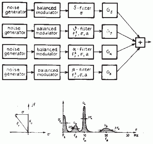 Figure 56.3 Block diagram of the EEG simulator; the θ filter represents a first-order active RC network; the ω, α, and β filters are of second order; potentiometers independently control the parameters f(2/r) (which determine the resonance frequency f0), σ (which determine the bandwidth), and α (which determine the zero of the transfer function); the power parameter is G. (Adapted from Zetterberg LH. Experience with analysis and simulation of EEG signals with parametric description of spectra. In: Kellaway P, Petersen I, eds. Automation of Clinical Electroencephalography. New York, NY: Raven Press; 1973:161-201.) |
Isaksson and Wennberg (22) concluded that, for most practical applications, a SPA model of the fifth order, at the highest, is sufficient, although using this order model only the first-order delta component and the second-order alpha and beta components can be described. In a few cases, it may be necessary to use a model of the seventh order to include a second-order theta component. In a study comparing the degree of visually evaluated slow activity in a large number of artifactfree EEG epochs with the features identified through SPA of the same epochs, Isaksson and Wennberg (23) concluded that, for most derivations, there was a significant linear correlation between the degree of slow activity encountered with visual inspection and the value of the features Gω (positive correlation) and σω (negative correlation); in a few cases, there was also correlation with Gα (negative correlation) and σα (positive correlation). The computation of an ARMA or AR model yields an important degree of data reduction. The relevant information is thus condensed in the coefficients of the model; the number of coefficients corresponds to the order of the model. As shown by Mathieu et al. (24) and Jansen (25), the coefficients can be used to characterize the EEG directly. The importance of this approach for EEG pattern classification is discussed later.
The Recognition and Elimination of Artifacts: Eye Movements and Muscle Artifacts
Physiologic and technical artifacts are the outstanding enemies of automatic EEG analysis. They must be eliminated if computer EEG analysis is to be used in clinical practice. It is a general requirement of EEG recording in any clinical laboratory that the records have a minimum of technical artifacts, a requirement that is even more critical in automatic analysis. One way to control the quality of EEG signals while performing analog-to-digital conversion in the clinical laboratory is by simply deleting those epochs that are below acceptable standards due to technical or to physiologic (e.g., ocular or muscular) artifacts. For example, the technician responsible for this operation may delete the series of digitized samples immediately preceding an identified artifact. Nevertheless, there will always be situations in which artifacts, particularly those of a physiologic nature, are unavoidable. This is particularly important during long-lasting EEG monitoring in several clinical (e.g., EEG-video monitoring of epileptic patients) and experimental (e.g., sleep studies) conditions and when computer-assisted quantification is applied (see also Chapter 35).
Eye movements and muscle potentials occur in most records of a few minutes’ duration; they can distort power spectra and lead to detection of transient nonstationarities that may be difficult to distinguish from epileptiform events. Eye blinks can be reduced by recording with eyes closed; slow eye movements, however, are more difficult to avoid. These are bilaterally synchronous with a maximum in frontal derivations and represent an important contribution to the power in the delta band in these derivations. In the early days of EEG quantification, Gotman (6) discussed several methods of avoiding this type of artifact at the very first stage, for example, by subtracting the electro-oculogram (EOG). This matter has been reviewed by Jervis et al. (26) and by Brunia et al. (27). However, the technique of EOG subtraction may give rise to distortion of the EEG signals, since the EOG recording also contains brain signals (28) that may be partially eliminated by filtering first the EOG with a low pass of about 8 Hz. The transfer of EOG activity to the EEG can be analyzed using a frequency domain approach. Eye blinks and slow eye movements have different spectral properties and are transferred in different ways to the skull. Gain functions for transferring both types of eye movements to the skull were computed by Gasser et al. (29). These authors obtained average gain functions that they found to be of practical use in correcting EOG artifacts. In other studies, a frequency domain approach to correcting EOG artifacts has been proposed (30,31). Similarly, Jervis et al. (32) found that a computerized correlation technique provides results superior to analog techniques for removing eye movement artifacts. Elbert et al. (33) also stressed that the best correction for these
types of artifacts is obtained in the frequency domain, but indicated that the correction procedure should be based on more than one EOG derivation, and preferably on three. Fortgens and de Bruin (34) also obtained good results using the method of least squares based on four EOG derivations.
types of artifacts is obtained in the frequency domain, but indicated that the correction procedure should be based on more than one EOG derivation, and preferably on three. Fortgens and de Bruin (34) also obtained good results using the method of least squares based on four EOG derivations.
Other important physiologic artifacts are muscle potentials. Here also it is important to note that electromyographic (EMG) signals affect the EEG power spectrum not only at relatively high frequencies (30 to 60 Hz) but also even down to 14 Hz (35). Under normal conditions, there is very little EEG power at the scalp in the 30- to 50-Hz band; if the power is significantly large, however, one must suspect contamination with EMG signals. Gotman (6) proposed dealing with this problem by introducing a reduction factor with which the activity in the beta band should be multiplied; this factor depends on the spectral intensity integrated over the 30- to 50-Hz band. If this is below 1.5 µV/Hz, the reduction factor is equal to unity; if the activity is larger than 1.5 µV/Hz, the reduction factor decreased linearly to 0.1 as the spectral activity increases up to 5.0 µV/Hz.
An alternative way to deal with artifacts is that used by Gevins et al. (36), who determined thresholds for head and body movement artifacts (under 1 Hz), high-frequency artifacts mainly caused by EMG (34 to 50 Hz), and eye movements (below 3 Hz in frontal derivations) based on a short segment that includes those artifacts; thereafter, EEG epochs exceeding the aforementioned thresholds were simply discarded (37).
The need to avoid the contamination with artifacts of relevant EEG features is so pressing that this area of EEG signal analysis has been, for decades, in constant evolution. Here we briefly review the most relevant approaches.
Rather elaborate methods are based on decomposing a set of EEG signals into components that should represent the artifact and the EEG signals, respectively. One of these is the spatial filtering approach (38,39). According to this method, the topography of the artifact is first estimated on the basis of a specific recording where the artifact is clearly evident, since this is, in general, easier to model than the EEG. Thus, the artifact can be described as the product of the corresponding topography vector and time waveforms. This can be then subtracted from the EEG signals contaminated with artifact to yield the corrected signals.
Other methods have been proposed that differ in the way of separating EEG and artifact signals. With this objective Lagerlund et al. (40) used principal component analysis (PCA), but this method has the drawback that PCA yields uncorrelated components while the EEG signals and the artifacts may be correlated. An important step forward in this context has been the introduction of independent component analysis (ICA) (see Chapter 54) that is very effective in separating EEG signals from artifacts as shown in a number of applications (41, 42, 43 and 44). The application of ICA, however, needs some form of postprocessing to identify the components corresponding to the EEG signals and to the artifacts. Several strategies and combinations of approaches particularly with respect to their practical implementation are discussed by Ille et al. (38) and by Makeig et al. (42). Particularly useful is the software package developed by Makeig’s group (45,46) that they called EEGLAB. This is an interactive Matlab toolbox for processing continuous and event-related EEG, magnetoencephalogram (MEG), and other electrophysiologic data using ICA, time/frequency analysis, and other methods including artifact rejection, as indicated below.
Transient Nonstationarities: Epileptiform Events
The detection of epileptiform events is a typical example of the application of a pattern recognition approach in EEG analysis. In this case, the epileptiform events (spikes, sharp waves, and spike-and-waves) are considered to constitute the “signal,” whereas the background activity constitutes the “noise.” The difficulty here lies in defining the epileptiform transients, that is, the “signals” that one wants to identify. In 1949, Jasper and Kershman (47) classified these events into spikes (duration 10 to 50 milliseconds) and sharp waves (duration 50 to 500 milliseconds). The Terminology Committee of the International Federation of EEG Societies defined spikes as waves with a duration of 1/12 second (83 milliseconds) or less, and sharp waves as waves with a duration of more than 1/12 second and less than 1/5 second (200 milliseconds) (48). Later, this Federation Committee gave somewhat different duration limits for these phenomena, with spikes having a duration from 20 to under 70 milliseconds and sharp waves having a duration of 70 to 200 milliseconds (49). A few other characteristics have been identified. Spikes and sharp waves should be clearly distinguishable from background activity and have a pointed peak; their main component should be generally negative relative to other scalp areas, and their amplitude variable. A distinction between spikes and sharp waves has descriptive value only. The parameter characteristics of spikes found in the human EEG have been studied by Celesia and Chen (50).
One problem is the difficulty of defining a learning set that may be unambiguous. A pioneering investigation in this respect was carried out by Gose et al. (51); this study revealed considerable intra- and interrater variability. In practical terms several methods have been used to identify the epileptiform events by increasing the signal-to-noise ratio. Most of them are akin to the classic approach of Carrie (52), who used as a criterion the ratio between the amplitude of the second derivative of the EEG signal and the moving average of similar measurements from a number of preceding and consecutive waves; a ratio of 4 or 5 was said to indicate an epileptiform event. Most other relevant studies have proposed similar types of measures (53, 54, 55, 56 and 57). All these methods involve a preprocessing stage that constitutes a form of high-pass filtering (e.g., computing the signal’s second derivative).
The method used by Lopes da Silva et al. (58, 59, 60, 61 and 62) is based on an essentially more general form of preprocessing. In this method, an EEG epoch is described by way of an AR model that provides the best fit to the background activity. The basic operation to improve the signal-to-noise ratio consists of passing the EEG signal through the inverse filter of this estimated AR model; this inverse filtering operation yields a new signal that ideally should have the properties of uncorrelated white noise. The statistical properties of this new signal are then determined; deviation of the new signal resulting from inverse filtering from a normal distribution at a certain probability level is thought to identify a transient nonstationarity (see Fig. 54.14). The essential feature of this method is that inverse filtering of the EEG epoch eliminates in an optimal way the background activity, allowing the transient nonstationarities to emerge clearly.
Not all transient nonstationarities, however, are necessarily epileptiform events; some may be physiologic artifacts or other kinds of EEG transients (e.g., lambda waves or sharp bursts of alpha waves). After detecting transient nonstationarities, one must apply a form of pattern recognition to select those that can be accepted as being epileptiform in nature. This constitutes the “two-stage analysis approach” proposed by Guedes de Oliveira and Lopes da Silva (63) and Guedes de Oliveira and Lopes da Silva (64). Two main pattern recognition methods have been proposed; one is based on a matched filtering approach and the other on piecewise characterization of the transient. Matched filtering using as template a spike-and-wave pattern has been used (65) to detect epileptiform transients even without preprocessing. Barlow and Dubinsky (66) used a comparable method, computing the running correlation coefficient between the EEG signal and a template (see Fig. 54.15). However, the variability of the waveforms characteristic of such transients presents a serious difficulty in dealing with this problem in practice. Pfurtscheller and Fischer (67) combined a preprocessing stage using inverse autoregressive filtering and a template matching stage for postselection of relevant epileptiform events. An alternative method is to apply a piecewise analysis to the transient nonstationarities, to identify those that belong to the epileptiform class. Smith (68) and Ktonas and Smith (69) proposed such a piecewise analysis method based on five features (Fig. 56.4): S1 and S2, the maximum slopes, respectively, before and after reaching the peak of the spike; S3, the time taken by the spike to reach the peak after it attains maximum slope; and S4, the time taken by the spike to reach maximum slope after the peak. The sum (S3 + S4) of the time intervals corresponds to the duration of the epileptiform spike (S5). The interval between two consecutive zero crossings of the same polarity of the first derivative (S6) is also a relevant feature.
Frost (70) considered the problem in a simpler form, proposing the following characteristic features. Assuming that an epileptiform spike is a triangular wave with a point of origin M at the base, an apex S, and a point of termination P, Frost defined amplitude as the largest value of the segments MS or SP, and duration as the interval MP. Furthermore, he used as a measure of sharpness D, an estimate of the signal’s second derivative. The initial processing step involves comparing the value of D with a threshold, so that, whenever D is larger than a certain value, a candidate spike is detected. Extracting the features described here requires a relatively high rate of EEG sampling—at least 200/sec.
The next section considers the practical implications of these methods in assessing the EEGs of epileptiform patients. According to the method of Gotman and Gloor (55), at the end of an analysis session the computer displays all transients detected, whether true or false. The distinction between these two types is made off-line in an interactive way. This form of analysis represents a considerable data reduction and provides a reliable account of the main types of epileptiform transients present in a given record.
The methods of analysis described in this section not only are useful in detecting the presence of epileptiform events, but also provide quantitative information on the morphology of such events, on their distribution over long periods of time, and on their spatial distribution. Using this methodology, Ktonas and Smith (69), Lopes da Silva et al. (1978), and Gotman (71) observed that most epileptiform spikes, at the scalp, present a second slope that is steeper than the first, contrary to the qualitative description of Gloor (72). However, Lemieux and Blume (73) found that the spikes recorded directly from the cortex presented a first slope that was equal or steeper than the second. Another interesting analysis that can be realized using these methods consists of the quantification of the distribution of epileptiform spikes in relation to the occurrence of seizures. Gotman and Marciani (74) found that the level of spiking is not related to the probability of seizure occurrence, but they reported an increase in spiking in the days following seizures.
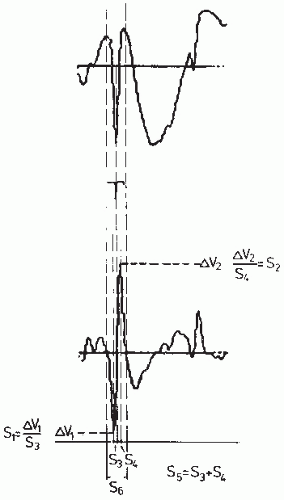 Figure 56.4 Top: An epileptiform spike; bottom: the corresponding first derivative. The parameters proposed by Ktonas and Smith (69) are shown: S1 and S2, the maximal spike slopes, respectively, before and after reaching the peak; S3, the time taken by the spike to reach the peak after it attained maximal slope; S4, the time taken by the spike to reach maximal slope after the peak. The sum S3 = S3 + S4 is a measure of the duration of the sharp part of the peak. The time interval between two zero crossings of the same polarity of the first derivative is S6. The time duration of the signal shown is 1 second. (Adapted from Lopes da Silva FH. Analysis of EEG nonstationarities. Electroencephalogr Clin Neurophysiol Suppl. 1978;34:163-179.) |
Very much as in the case of the detection of artifacts, the analysis of epileptiform events has attracted the interest of many researchers and new approaches are often being introduced. In most cases, new methods are published without a comprehensive comparison with older methods, which make it difficult to evaluate the performance of new approaches with respect to previous ones. An interesting exception is the study
of Dumpelmann and Elger (75), which we discuss in detail below (see the section “CADS and Epileptiform Events”).
of Dumpelmann and Elger (75), which we discuss in detail below (see the section “CADS and Epileptiform Events”).
Very often several categories of spikes can be distinguished in the EEG or MEG of patients with epilepsy that may differ considerably in waveform and may even be associated with different sources in the brain. Therefore, the population of spikes recorded in a given patient should preferably be grouped into distinct categories before being averaged. This is especially relevant if source reconstruction is going to be performed. This implies that a form of clustering of spikes has to be carried out. In the simplest case, this may be done by visual inspection by an experienced electroencephalographer. Such an operation becomes rather complex and time consuming if the number of spikes and of channels in the EEG/MEG is quite large. This has led to the development of computer algorithms to automate the identification of clusters of spikes (76). We should add that if the purpose of the analysis of epileptiform spikes includes the estimation of the localization of the corresponding sources in the brain, it is preferable to use MEG than EEG recordings because solutions of the inverse problem are more accurate with MEG (see also Chapter 5). One of these studies is that of Van’t Ent et al. (77) who performed cluster analysis of MEG epileptiform spikes, grouping spikes according to the similarity between magnetic field characteristics. Thereafter, the spikes within one cluster are averaged to improve the signal-to-noise ratio such that the quality of equivalent dipole source estimates is enhanced. Similarly Abraham-Fuchs et al. (78) showed that averaging of similar spike events, recorded in the MEG, substantially improves the signal-to-noise ratio (a more general discussion of clustering algorithms is presented in the next section).
Classification and Clustering in EEG Analysis
The previous section considers different ways to find sets of features that can characterize EEG signals. In this section, we consider very briefly the next phase in pattern recognition, classification and/or clustering. For a detailed account of this problem, the reader is referred to Duda and Hart (1) as indicated above. It is necessary to consider this question here in order to be able to evaluate quantitative EEG analysis methods in the clinical laboratory. The essential problem is one of diagnosis; given a set of EEG epochs that have been analyzed and characterized by a number of features, it is necessary to determine what is the performance of the algorithm regarding the classification of the EEG epochs in a given number of diagnostic categories (e.g., normal/abnormal, sleep stages) or to label EEG transients (e.g., spikes) as epileptiform.
One way to solve this problem is to use discriminant analysis, which is possible only if one knows a priori that the EEG signals belong to a defined number of classes. Assuming that the analysis involves classifying EEG signals into two classes, normal and abnormal, and using a set of features, the feature vector defines a point in n-dimensional space.
In discriminant analysis, the space where all objects (e.g., EEG epochs characterized by a vector set) are contained must be subdivided into a number of regions; the objects within a region form one class. The functions that generate the surface separating the regions are called discriminant functions. An object is assigned to a certain region or class by several types of decision rules; these are described in detail by Demartini and Vincent-Carrefour (4), among others.
To develop and test a classifier, it is important to dispose of a sufficiently large learning set (i.e., a set of N objects that have been classified a priori using independent criteria); in the case of EEG analysis, the independent criteria ought to be clinically valid. This implies that the objects must be classified by expert raters (electroencephalographers) using generally accepted criteria, possibly based on visual inspection, and making use of all relevant clinical information. The learning set should contain a sufficient number of objects (4). One way to develop an automatic method of EEG analysis is to divide the experimental set into two parts. Thus, the first part (learning set) is used to develop the classifier and the second to test its performance (test set). A useful alternative if the experimental set is too small is the “hold-one-out” strategy, which involves removing one object from the learning set and then resynthesizing the classifier and trying to recognize the selected object. This operation should be repeated for each object. The resulting error rate is a good estimate of the classifier’s performance.
The quality of the learning set is of primary importance. To start with, it is necessary to have knowledge about rater reproducibility (intrarater agreement) and validity (interrater agreement) as regards evaluation of the EEG records constituting the learning set. A few studies have addressed electroencephalographers’ overall classification of EEG records as normal or abnormal; in such cases, the validity of the visual assessment is usually about 80% to 90%. Although most raters generally agree on the division of the EEG into two classes globally (normal or abnormal), classification of short segments or of epileptiform transients is much less consistent. The same applies to intrarater agreement. In the assessment of EEG patterns corresponding to different sleep stages, however, a good degree of interrater agreement can be expected; thus, it is not surprising that methods of automatically classifying sleep stages have been those more often evaluated in a quantitative way. In assessing epileptiform events (spikes, sharp waves, spikes-and-waves), a large degree of interrater variability is also encountered. Gose et al. (51) found considerable variability in the human detection of spikes; a total of 948 events were marked as spikes by one or more electroencephalographers, but only 104 events were marked by five raters. However, disagreement between raters on individual spikes is not very important; a comparison on a patient basis (30 records seen by five raters) is more important; seen from this viewpoint, the average error rate was only 4%.
For the classification of EEG records in the learning set, it is important to utilize a structural report such as used by Volavka et al. (79), Rose et al. (80), Gotman et al. (81), Gotman and Gloor (55), and Gevins (82). In other words, EEG classes should be defined unambiguously; the abnormal EEG can be classified as paroxysmal or irritative, hypofunctional (cortical or centrencephalic) or mixed; the location of the abnormality (focal: frontal, temporal, central, occipital, lateralized, or diffuse) should also be specified. Furthermore, one may use a complementary second-order classification into diagnostic types related to the global medical diagnosis: space-occupying lesions, metabolic disorders, cerebrovascular insufficiency, seizure disorders, or psychiatric disorders.
EEG SEGMENTATION AND CLUSTERING
We should emphasize that EEG records are generally nonstationary. Although in the clinical laboratory it is usually possible to obtain representative EEG epochs by tightly controlling the subject’s behavioral state, it is often desirable to distinguish in an EEG signal segment, characterized by different properties, that can be separated automatically. This is particularly important in the case of EEGs recorded under intensive care conditions, such as during anesthesia, or in other long-duration records. Ideally equivalent segments thereafter could be grouped together, thus defining a number of classes. An early effort in this direction was made by Bodenstein and Praetorius (83), who proposed a general method of EEG segmentation; they assumed that an EEG should be considered as a sequence of quasi-stationary segments of varying duration. They used an AR model as described in Chapter 54.
By setting appropriate thresholds, Bodenstein and Praetorius (83) have been able to formulate explicit criteria for EEG segmentation. The problem, however, is that the validity of this segmentation procedure in relation to clinically clearly defined states is difficult to demonstrate. Jansen (25) made an interesting effort along a similar line by using an algorithm akin to that discussed above but based on a Kalman filter and following a different strategy; this method is called Kalman-Bucy (KB) clustering. Defining segments of variable length based on statistical criteria proved to be too difficult because a good learning set could not be constructed. An alternative method followed by Jansen (25) was to divide the EEG into a large number of segments with a fixed duration of 1.28 seconds each, and classified them using an unsupervised learning clustering approach. In other words, he used a clustering algorithm to group segments with similar properties into a number of classes that were not defined a priori. Each 1.28-second segment is characterized by a feature vector consisting of the five coefficients of the corresponding AR model estimated using a Kalman filter, often complemented by a measure of amplitude. The statistical approach used in this case is a form of clustering (see review in Ref. 84). Clustering can be partitional or hierarchical; the former is based on a priori knowledge of the place occupied by some objects, which are then used as “seed points” around which clusters grow. The latter can have two forms, agglomerative or divisive, depending on whether one starts from an assembly of as many clusters as objects or from one cluster encompassing all objects. Jansen (25) used the agglomerative hierarchical clustering approach to group EEG segments of a number of types. This type of clustering involves an iterative process through which the two most similar clusters of the previous step are merged into a new cluster. The user can stop the process at any point, depending on the application. Using statistical criteria, it is possible to delimit the number of classes in such a way that the distance between their centroids does not fall below a certain value.
Related posts:


Stay updated, free articles. Join our Telegram channel

Full access? Get Clinical Tree


