EEG Mapping and Source Imaging
Christoph M. Michel
Bin He
INTRODUCTION
This chapter is concerned with the use of EEG as a functional imaging method. Great advancements have been made in the past several years in recording and analyzing of high-resolution EEG. Powerful EEG systems have been designed that allow fast and easy recording from hundreds of channels simultaneously, even in clinical settings. Sophisticated pattern recognition algorithms have been developed to characterize the topography of the scalp electric fields and to detect changes in the topography over time and between experimental or clinical conditions. New methods for estimating the sources underlying the recorded scalp potential maps have been constructed and applied to numerous experimental and clinical data. The incorporation of anatomical information, as obtained from magnetic resonance imaging (MRI) in the individual subject, has boosted the use of electrophysiologic neuroimaging and has stimulated clinical interest.
We will here discuss these recent developments and present the current state of the art in electrophysiologic neuroimaging, thereby extending other recent detailed reviews on this topic (1, 2, 3, 4, 5 and 6).
Neuronal activities in the brain generate current flows in the head volume conductor, reflected as electric potentials over the head surface, where they give rise to a specific topographical map. The proper recording and analysis of these maps are precursors for source localization. A great deal of localization information can already be derived from these maps, but their incorrect interpretation can also lead to a misleading conclusion about the putative generators. The second section of this chapter will deal with the proper recording of the scalp potential fields and the characterization, description, and statistical comparison of scalp potential maps. It will also summarize analysis methods that are based on spatiotemporal characteristics of potential maps, thereby leading to data reduction and a priori constraints for subsequent source localization.
The propagation of the electric potential in the brain that is generated by the active neuronal populations is modulated by the conductivity properties of the different tissues and by the shape of the head. If these parameters are known, the electric potentials that a given current source in the brain produces on the surface electrodes can be calculated. This so-called forward solution is the basis of every source localization method. The third section of the chapter will discuss the different head models and the current knowledge on head conductivities and their influence on the scalp potential maps.
EEG source localization has evolved from single dipole searching methods to distributed source estimation procedures without any a priori assumption on the number of sources. However, solving the underdetermined inverse problem requires a priori assumptions based on information other than the number of sources, preferentially incorporating physiologic or biophysical knowledge. The correctness of these assumptions determines the correctness of the source estimation. The fourth section will discuss the different source reconstruction algorithms that are currently used and show examples of applications.
The spatial resolution of high-density EEG with sophisticated source localization methods in realistic geometry head models has become very impressive and the images that are produced are as tempting as pictures from other functional imaging methods, particularly because they show direct neuronal signaling rather than indirect metabolic changes. But EEG has a second important attraction: the high temporal resolution. This temporal resolution combined with electrophysiologic neuroimaging leads to the possibility to elucidate the temporal dynamics of neuronal signaling in large-scale neuronal networks and directly estimate network connectivity. The last section will discuss such analysis methods.
The power of EEG as a functional neuroimaging method is largely underestimated and many impressive experimental and clinical studies using these tools have not received the attention they merit. The reason is manifold. First, functional MRI has received a unique status of being able to reduce brain activity to the underlying sources nonambiguously. Second, misinterpretations of EEG and evoked potential waveforms due to a lack of understanding of the properties of electromagnetic fields, of the role of the reference electrode, and of the influence of nonneuronal signals such as myogenic or occulomotor activity resulted in a number of claims that later proved to be wrong. Third, the EEG is somehow harmed by history. The term EEG is still often related to the artistic interpretation of graph elements by some skilled neurophysiologists. The magnetoencephalogram (MEG) that basically measures the same neuronal activity with the same limitations does not suffer from this history and is easily considered as a neuroimaging method by public encyclopedias such as Wikipedia. With this chapter we would like to diminish this incorrect historical view and show that the EEG has considerably matured and can now be considered as a powerful, flexible, and affordable imaging technology.
MAPPING OF THE SCALP ELECTRIC FIELD
Electrophysiologic neuroimaging is based on the recording of the electric potential from a multitude of electrodes distributed over the surface of the head. From these simultaneous recordings a
potential map can be constructed for any single moment in time, depicting the momentary configuration of the potential field (7). The idea to analyze these topographies instead of waveform morphologies has already been formulated some decades ago (8, 9 and 10) and has been called EEG topographical mapping. EEG mapping is a precursor to source imaging (11), and the proper analysis and interpretation of EEG maps can give a great deal of information with regard to the putative sources in the brain. Most importantly, by physical laws, different map topographies must have been produced by different source configurations in the brain (12). Thus, statistical methods that allow determining significantly different map topographies over time or between conditions or subjects provide important a priori hypotheses about whether and when differences in the source localization algorithms can be expected. Analysis of topographic maps is therefore an important step in electric source imaging (3).
potential map can be constructed for any single moment in time, depicting the momentary configuration of the potential field (7). The idea to analyze these topographies instead of waveform morphologies has already been formulated some decades ago (8, 9 and 10) and has been called EEG topographical mapping. EEG mapping is a precursor to source imaging (11), and the proper analysis and interpretation of EEG maps can give a great deal of information with regard to the putative sources in the brain. Most importantly, by physical laws, different map topographies must have been produced by different source configurations in the brain (12). Thus, statistical methods that allow determining significantly different map topographies over time or between conditions or subjects provide important a priori hypotheses about whether and when differences in the source localization algorithms can be expected. Analysis of topographic maps is therefore an important step in electric source imaging (3).
Visualization and proper inspection of topographic maps is also mandatory for source imaging to assure that maps that are clean of artifact enter the algorithms. The quality of the maps determines the goodness of the source imaging procedures. It is therefore of crucial importance that these scalp potential fields are recorded and preprocessed in a reasonable manner, and that they are visualized and carefully inspected before applying source imaging algorithms to them. This particularly concerns EEG that is recorded in noisy environments such as in the MRI scanner. EEG waveforms that look correct after filtering and denoising do not yet necessarily indicate that the EEG maps will be correct and usable for source analysis.
In the following we discuss some practical issues related to the recording and construction of topographic maps. This concerns the number and the distribution of the electrodes on the scalp to provide an adequate spatial sampling of the potential field. It also concerns the parametric description of the map configuration and the comparison of map topographies in a global and reference-independent way. Further details can be found in Ref. 13.
Spatial Sampling
It is clear that proper sampling of the electromagnetic field over the whole scalp needs a large number of sensors. The MEG community has consequently quickly moved from low- to high-resolution systems, and most of the MEG laboratories are nowadays recording from over ˜150 channels. Until recently, this was a severe limitation for the EEG, because application of a large number of electrodes was time consuming, uncomfortable, and expensive. However, this is not a limiting factor anymore. EEG systems of up to 256 electrodes are commercially available and are easy and fast applicable, even in clinical settings (Fig. 55.1) (14, 15, 16 and 17).
The question of how many electrodes are needed for proper EEG mapping and source imaging is not completely answered. It depends on the spatial frequency of the scalp potential field, which is limited by the blurring caused by volume conductor effects, particularly induced by the low conductivity of the skull (18). The maximal spatial frequency has to be correctly sampled to avoid aliasing, which appears when the frequency of the measured signal is higher than the sampling frequency. In the case of discrete sampling of time-varying signals, a sampling frequency that is twice as high as the highest frequency in the signal is required to avoid aliasing (Nyquist rate) (see also Chapter 54). Similar rules apply to sampling in space, since the potential distribution is only sampled at discrete measurement points (electrodes) (19,20). Spatial frequencies of the potential field that are higher than the spatial sampling frequency (i.e., the distance between electrodes) will distort the map topography (21, 22, 23 and 24) and will lead to misinterpretation of maps and consequently to mislocalization of the sources.
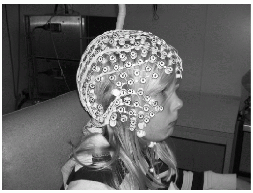 Figure 55.1 High-resolution EEG. Example of an EEG system that allows fast application of 256 electrodes. The electrodes are interconnected by thin rubber bands and each contains a small sponge that touches the subject’s head directly (14). The nets are soaked in saline water before put on the subject’s head. The whole net is applied at once and needs no skin abrasion and no electrode paste. (HydroCel Geodesic Sensor Net constructed by Electrical Geodesics Inc., Eugene, OR, USA.) |
Already many years ago, researchers tried to estimate the maximal spatial frequency of the scalp electric field based on theoretical considerations and modeling. These works suggested that interelectrode distances of ˜2 to 3 cm are preferable (25,26) for proper sampling of the field, which would lead to around 100 required electrodes. Freeman et al. (27) suggested from spatial spectral density calculations that even less than 1-cm spacing of electrodes is needed. Lantz et al. (28) and Michel et al. (3) performed simulations using dipole forward modeling (see section “EEG Forward Problem”) to calculate the dipole localization error of different source localization algorithms when different number of electrodes were used. Both studies showed that the localization precision does not increase linearly, but reaches a plateau at about 100 electrodes for fully distributed inverse solution algorithms.
Several experimental studies used subsampling techniques to establish the number of electrodes needed to correctly reconstruct potential maps and localize the sources. Michel et al. (3) demonstrated incorrect lateralization of the source estimated for the P100 component of the visual-evoked potential when downsampling from 46 to 19 electrodes, and that an incomplete coverage of the scalp surface can lead to complete misplacement of the sources (Fig. 55.2). Luu et al. (29) and Lantz et al. (28) used the
downsample method in clinical data to evaluate the correctness of localization of pathologic activity. Luu et al. (29) studied patients with acute focal ischemic stroke recorded with 128 electrodes and downsampled to 64, 32, and 19 channels. Visual comparison of the EEG maps with radiographic images led to the conclusion that more than 64 electrodes were desirable to avoid mislocalizations of the affected region. More objectively was the downsample study of Lantz et al. (28) on 123-electrode recordings from patients with partial epilepsy. Fourteen patients with different focus localization were recorded before successful resective surgery; thus, the location of the epileptic focus was known. Several interictal spikes were manually identified and then downsampled to 63 and 31 electrodes. Source localization was applied to each single spike and the distance of the source maximum to the resected area was determined and statistically compared between the different electrode sets. Significant smaller localization error was found when using 63 instead of only 31 electrodes. Accuracy still systematically increased from 63 to 123 electrodes, but less significantly (Fig. 55.3).
downsample method in clinical data to evaluate the correctness of localization of pathologic activity. Luu et al. (29) studied patients with acute focal ischemic stroke recorded with 128 electrodes and downsampled to 64, 32, and 19 channels. Visual comparison of the EEG maps with radiographic images led to the conclusion that more than 64 electrodes were desirable to avoid mislocalizations of the affected region. More objectively was the downsample study of Lantz et al. (28) on 123-electrode recordings from patients with partial epilepsy. Fourteen patients with different focus localization were recorded before successful resective surgery; thus, the location of the epileptic focus was known. Several interictal spikes were manually identified and then downsampled to 63 and 31 electrodes. Source localization was applied to each single spike and the distance of the source maximum to the resected area was determined and statistically compared between the different electrode sets. Significant smaller localization error was found when using 63 instead of only 31 electrodes. Accuracy still systematically increased from 63 to 123 electrodes, but less significantly (Fig. 55.3).
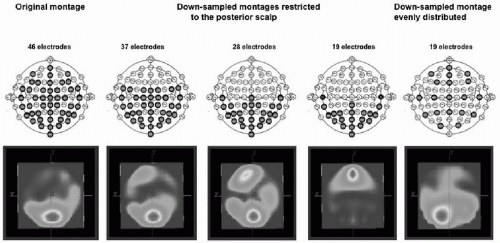 Figure 55.2 Spatial sampling. The figure illustrates the importance of proper sampling of the scalp potential field. Visual-evoked potentials were recorded from 46 electrodes positioned according to the scheme on the left. A distributed source localization algorithm (LORETA) was applied to the data at the peak of the P100 component, resulting in a medial occipital source maximum. Data were then downsampled to fewer electrodes that were restricted to the posterior part of the head. The same localization procedure (with the same spherical head model) at the same time point led to incorrect localization, with even a frontal maximum with 19 occipital electrodes. Using again only 19 electrodes, but distributing them equally over the head as illustrated on the scheme on the right, leads to a complete sampling of the electric field and to a more correct localization. (From Michel CM, Lantz G, Spinelli L, et al. 128-Channel EEG source imaging in epilepsy: clinical yield and localization precision. J Clin Neurophysiol. 2004;21:71-83.)(See color insert) |
The above-described studies estimate that around 64 or more electrodes are desirable for accurate spatial sampling and reconstruction of the scalp potential field. However, as shown by Ryynänen et al. (23,24) in computer simulation studies, these estimations are only valid if we assume a conductivity ratio of approximately 1:80 between skull and brain, as proposed by Rush and Driscoll (30). These traditional values were used in the above-described simulation and downsampling studies, but they are most probably incorrect as indicated by several recent studies (31, 32 and 33). If the conductivity of the skull is lower as it is proposed by these studies, the spatial blurring is smaller and the spatial frequency is higher. Ryynänen et al. (23,24) investigated the relation between the number of electrodes and the resistance values of the different compartments. Their computer simulation results suggest that if the 1:80 ratio is considered as correct, 64 to 128 electrodes are indeed sufficient. However, when more realistic skull conductivity values are used, a higher number of electrodes may be needed. More realistic values for the conductivity ratio are suggested to be between ˜20 and 50 (34), depending on the skull thickness. In an experimental study of pediatric patients undergoing intracranial recordings, He and colleagues (35) measured the scalp and subdural potentials simultaneously during cortical current injection, and used them to estimate the brain-to-skull conductivity ratio. The experimental data suggested that the averaged brain-to-skull conductivity ratio is about 25 when using the three-sphere head model (33), and about 20 when using the realistic geometry finite element head model (35). In newborns the skull thickness is approximately seven to eight times lower than in adults, leading to a ratio of approximately 14:1 (20,36). Ryynänen et al. (24) suggested from their computer simulation studies that with this ratio, spatial resolution still increases with
256 as compared to 128 electrodes in realistic noise levels. Grieve et al. (20) also suggested that a 256-electrode array is needed in infants to obtain a spatial sampling error of less than 10%. However, larger electrode arrays are also more influenced by measurement noise, which affects the spatial resolution. As suggested by Ryynänen et al. (23,24), the measurement noise is a critical limiting factor for the spatial resolution of high-density EEG systems. Thus, there is an important interplay between number of electrodes, measurement noise, and conductivity values of the different compartments of the head. Furthermore, it remains for the moment unclear how much an imperfect spatial sampling influences the source imaging. Some data did suggest that even with ˜32 electrodes, one gains important insight about the underlying brain electric sources by performing source localization and imaging (37, 38, 39 and 40). Further studies with direct measurements of the conductivities at different locations on the head through current injection (41) or with the aid of MRI (42) will be needed to definitely answer the question of the head tissue conductivity. Further experimental and clinical studies shall also be needed to systematically investigate the question of optimal number of electrodes that are needed to recover spatial features of scalp topography and to estimate the underlying brain sources that generate the scalp EEG.
256 as compared to 128 electrodes in realistic noise levels. Grieve et al. (20) also suggested that a 256-electrode array is needed in infants to obtain a spatial sampling error of less than 10%. However, larger electrode arrays are also more influenced by measurement noise, which affects the spatial resolution. As suggested by Ryynänen et al. (23,24), the measurement noise is a critical limiting factor for the spatial resolution of high-density EEG systems. Thus, there is an important interplay between number of electrodes, measurement noise, and conductivity values of the different compartments of the head. Furthermore, it remains for the moment unclear how much an imperfect spatial sampling influences the source imaging. Some data did suggest that even with ˜32 electrodes, one gains important insight about the underlying brain electric sources by performing source localization and imaging (37, 38, 39 and 40). Further studies with direct measurements of the conductivities at different locations on the head through current injection (41) or with the aid of MRI (42) will be needed to definitely answer the question of the head tissue conductivity. Further experimental and clinical studies shall also be needed to systematically investigate the question of optimal number of electrodes that are needed to recover spatial features of scalp topography and to estimate the underlying brain sources that generate the scalp EEG.
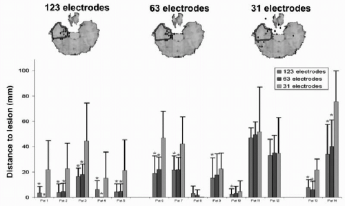 Figure 55.3 Influence of number of electrodes on source localization. Evaluation of source localization precision of interictal discharges in 14 epileptic patients, recorded with 123 electrodes. Single spikes were localized with a linear inverse solution in the individual brain and the distance of the source maximum to the resected area was measured. Mean and standard deviation of the distance were compared between the original high-resolution recording and with downsampling of the same data to fewer channels (but still equally distributed). The top row shows the example of one patient. The diamonds indicate the source maximum; the blue area marks the resected zone. Diamonds outside the brain are actually on another level and projected onto the illustrated slide. The bar graph shows the mean distance to the lesion. Stars indicate significant differences between the different number of electrodes. A clear significant amelioration of the localization precision was observed when increasing the number of recording channels. (From Michel CM, Brandeis D. Data acquisition and pre-processing standards for electrical neuroimaging. In: Michel CM, Koenig T, Brandeis D, et al., eds. Electrical Neuroimaging. Cambridge: Cambridge University Press; 2009. Modified after Lantz G, Spinelli L, Seeck M, et al. Propagation of interictal epileptiform activity can lead to erroneous source localizations: a 128 channel EEG mapping study. J Clin Neurophysiol. 2003;20:311-319.)(See color insert) |
Map Inspection, Artifact Correction, Interpolation
A mandatory requirement in EEG and ERP analysis is the detection and elimination of artifacts, caused by bad electrode contact, muscle or eye movement activity, or other environmental noise. Besides automatic detection of such artifacts using amplitude windows, careful visual inspection of the EEG traces is mandatory. These requirements evidently also hold for EEG mapping and source localization, but in addition to the need for clean EEG traces, the spatial EEG analysis also requires clean maps (13). Even if the EEG traces appear correct, they might be contaminated by noise that destroys the spatial configuration of the maps. Spatial inhomogeneities due to bad electrodes can drastically influence source localization outcome because they can lead to strong local gradients. Figure 55.4 illustrates this problem. In one case, the bad electrode is readily seen in the 256-channel EEG traces, and it is also easily seen in the topographic
map by a strong and isolated local potential minimum. The second bad channel is not easily seen in the traces and is not detected by an amplitude window. However, it is readily visible on the map by a negative “island” within the otherwise positive potential. Keeping these bad channels in the construction of the potential field leads to an incorrect estimation of a focal source under this electrode, which completely disappears when these electrodes are taken out.
map by a strong and isolated local potential minimum. The second bad channel is not easily seen in the traces and is not detected by an amplitude window. However, it is readily visible on the map by a negative “island” within the otherwise positive potential. Keeping these bad channels in the construction of the potential field leads to an incorrect estimation of a focal source under this electrode, which completely disappears when these electrodes are taken out.
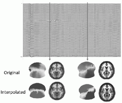 Figure 55.4 Influence of artifacts on source localization. Example of a 256-channel EEG recording and the reconstruction of the scalp potential map and the source estimation for this map using a distributed linear inverse solution (LAURA). The first time point (left) includes a clear artifact on a left temporal electrode, easily identifiable on the EEG traces and on the EEG map. This leads to a dominant source under this electrode position in the inverse solution. Excluding (or interpolating) this electrode leads to a dominant source on the contralateral temporal lobe. The artifact channel at the second time point (right) is not easily identifiable on the traces (artifact trace shown in red). However, the map clearly identifies this bad right frontal electrode with a negative potential surrounded by otherwise positive electrodes. Elimination of this bad electrode leads to a unique occipital source. Keeping the electrode for the inverse solution calculation leads to an additional right frontal source underlying this electrode. (Modified from Michel CM, Brandeis D. Data acquisition and pre-processing standards for electrical neuroimaging. In: Michel CM, Koenig T, Brandeis D, et al., eds. Electrical Neuroimaging. Cambridge: Cambridge University Press; 2009.)(See color insert) |
This example illustrates the importance of inspecting not only the EEG traces for abnormal graph elements, but also the potential maps for abnormal topographies. It is thereby important that the recording reference is included in the electrode array for map construction, because also the reference electrode is an active electrode and has to be inspected for abnormal values. The most convincing example has been demonstrated by Yuval-Greenberg et al. (43), showing a map with a very steep potential maximum at the nose reference. This was due to the recording of miniature saccades by this “noncephalic” reference electrode. This becomes readily visible when looking at the map, but is ignored and misinterpreted as occipital gamma activity when looking at single occipital electrodes that were recorded against this nose reference (43).
When data are averaged over sweeps or over subjects, bad electrodes must be interpolated before averaging. Most of the commonly used interpolation routines belong to the family of spline interpolations. Spline interpolations can be linear (based on a polynomial of first degree), or quadratic, cubic, or of higher order. Using cross-validation tests, it was concluded that higher order spherical spline interpolations perform reasonably well in sufficiently dense electrode arrays (44,45). The estimation of potentials is less reliable when the potentials are located outside of the electrode array and not between some electrodes. Extrapolating potentials beyond the electrode array should thus be avoided.
Efficient algorithms to detect and eliminate artifacts based on “abnormal” spatial configurations are increasingly used in EEG mapping and source localization studies. Most efficient are algorithms based on independent component analysis (ICA) (46). The ICA is particularly useful for eye movement artifact detection and elimination, because the artifact is largely independent from the remaining part of the data.
Topographic Analysis
The traditional analysis of EEG and evoked potentials relies on waveforms. Parameters of interest are thereby changes in amplitude or frequency, or peaks at certain latency time-locked to stimulus presentation. These measures are ambiguous because the EEG is by definition a bipolar signal. Changes of the location of one of the two electrodes will change the values of the above parameters. This ambiguity is well known and has led to a large discussion on the reference-dependency of the EEG and the question of the correct recording reference for a certain experimental or clinical condition (47, 48, 49, 50 and 51).
This reference problem of the EEG is completely resolved when topographic analysis methods are applied. The potential map topography does not depend on the reference (3,50,52, 53 and 54). The reference only changes the zero level, but the topographical features of the map remain unaffected (53). Thus, the reference only introduces a DC shift. This shift is eliminated when applying topographic analysis methods including source imaging. Elimination of the DC level can be achieved by calculating the so-called common average reference at each moment in time (9).
One way to sharpen the spatial details of the scalp potential maps is to calculate the scalp current source density, or the surface Laplacian of the potential (21,55,56). The surface Laplacian of the scalp potential is the second spatial derivative of the potential field in the local curvature in µV/cm2. The surface Laplacian has been mainly derived from unipolar potential recordings on the scalp, using algorithms such as finite difference algorithm (57), spherical spline algorithm (58), or realistic geometry spline algorithm (59). The surface Laplacian has been widely used in applications when one wishes to enhance the sensitivity to local activity. It can be interpreted as an estimation of the current density entering or exiting the scalp. It emphasizes superficial sources because deeper sources produce smaller potentials on the surface. Like the other topographic measures that will be described below,
the surface Laplacian estimates are independent of the position of the recording reference, because the potential common to all electrodes is automatically removed (60).
the surface Laplacian estimates are independent of the position of the recording reference, because the potential common to all electrodes is automatically removed (60).
Scalp potential maps can be characterized by their strength and their topography. A reference-independent measure of map strength is the global field power (GFP) (8). GFP is the standard deviation of the potentials at all electrodes of an averagereference map. It is defined as
where ui is the voltage of the map u at the electrode i,  is the average voltage of all electrodes of the map u, and N is the number of electrodes of the map u. Scalp potential fields with pronounced peaks and troughs and steep gradients, that is, very “hilly” maps, will result in high GFP, while GFP is low in maps that have a “flat” appearance with shallow gradients. GFP is a one-number measure of the map at each moment in time. Displaying this measure over time allows to identify moments of high signal-to-noise ratio, corresponding to moments of high global neuronal synchronization (61).
is the average voltage of all electrodes of the map u, and N is the number of electrodes of the map u. Scalp potential fields with pronounced peaks and troughs and steep gradients, that is, very “hilly” maps, will result in high GFP, while GFP is low in maps that have a “flat” appearance with shallow gradients. GFP is a one-number measure of the map at each moment in time. Displaying this measure over time allows to identify moments of high signal-to-noise ratio, corresponding to moments of high global neuronal synchronization (61).A reference-independent measure of topographic differences of scalp potential maps is the so-called global map dissimilarity measure (GMD) (8). It is defined as
where ui is the voltage of map u at the electrode i, vi is the voltage of map v at the electrode i, is the average voltage of all electrodes of map u,
 is the average voltage of all electrodes of map v, and N is the total number of electrodes. In order to assure that only topography differences are taken into account, the two maps that are compared are first normalized by dividing the potential values at each electrode of a given map by its GFP.
is the average voltage of all electrodes of map u, is the average voltage of all electrodes of map v, and N is the total number of electrodes. In order to assure that only topography differences are taken into account, the two maps that are compared are first normalized by dividing the potential values at each electrode of a given map by its GFP.The GMD is 0 when two maps are equal, and maximally reaches 2 for the case where the two maps have the same topography with reversed polarity. It can be shown that the GMD is equivalent to the spatial Pearson’s product-moment correlation coefficient between the potentials of the two maps to compare (62).
If two maps differ in topography independent of their strength, it directly indicates that the two maps were generated by a different configuration of sources in the brain (4,11,63). The inverse is not necessarily true: infinite number of source configurations may produce the same scalp potential topography (12). The GMD calculation is therefore considered as a first step for defining whether different sources were involved in the two processes that were compared. When comparing subsequent maps in time using the GMD, periods where source configuration changes appeared can be defined. It is interesting to note that the GMD inversely correlates with the GFP: GMD is high when GFP is low, that is, maps tend to be stable during high GFP and change the configuration when GFP is low (Fig. 55.5). The GMD is itself not a statistical measure. However, if two groups of maps are compared, a statistical statement of the significance of the topographic differences can be made. This is achieved by performing nonparametric randomization tests based on the GMD values as, for example, described in Ref. 54.
Spatiotemporal Decomposition
Source localization procedures can be applied to multichannel EEG and ERP data at any instant in time. With the high sampling rate of modern EEG systems that easily exceed 1000 Hz, this leads to a large amount of data from which the relevant information has to be extracted. Consequently, experimenters typically predetermine relevant events within a continuous time series of data to which source analysis will be applied. This particularly concerns ERP research, where peaks in certain time windows at certain electrodes are identified and spatially analyzed (64). This traditional approach is however less tenable with high-density EEG and ERP recordings, because different scalp sites have different peak latencies, and because the waveforms (and thus the peaks) at certain electrodes change when changing the position of the reference electrode.
An alternative to the traditional preselection of relevant events based on ERP waveforms is to define components on the basis of the topography of the potential field (65). Most commonly, some kind of spatial factor analysis methods are used for this purpose. These methods produce a series of factors that represent a weighted sum of all recorded channels across time. The aim of this factor analysis approach is to find a limited number of optimal factors that best represent a given data set. The load for each of these factors (i.e., the goodness of fit) then varies in time. Each factor represents a certain potential topography, that is, a prototypical map. Source localization applied to these maps results in a limited number of putative sources in the brain that explain a full time series of multichannel EEG data with time-varying strength.
The most commonly used variant of spatial factor analyses is the principal component analysis (PCA) (66, 67, 68 and 69). The first factor of the PCA solution accounts for the maximally possible amount of data variance, and each next orthogonal factor accounts for the maximum possible residual variance. Since factors that contribute little to the explained variance can be neglected, the PCA is a powerful exploratory tool to reduce complex multichannel EEG data in space and time. It has been repeatedly applied to ERP studies with the aim to extract ERP components whose variance is related to a given experimental condition. It can provide useful information on how a given experimental manipulation affects ERP components without any a priori assumption about the shape or number of components in the data set (69, 70, 71, 72 and 73).
The PCA does not allow for cross-correlations between activities corresponding to separate factors and thus excludes linear dependencies between the factor maps. However, it does not exclude dependencies based on higher order correlations. The factor analysis method that also removes these higher order relations is called independent component analysis (ICA) (74). The
objective of the ICA is sometimes illustrated by the so-called “cocktail party problem,” where the ICA allows decomposing a sound record from a party into the independent contributions of the individual persons. Like the PCA, the ICA produces a weight coefficient for each factor. Each factor is supposed to represent a temporally independent component.
objective of the ICA is sometimes illustrated by the so-called “cocktail party problem,” where the ICA allows decomposing a sound record from a party into the independent contributions of the individual persons. Like the PCA, the ICA produces a weight coefficient for each factor. Each factor is supposed to represent a temporally independent component.
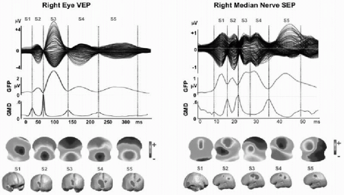 Figure 55.5 Spatial analysis of evoked potentials. Example of 256-channel visual-evoked potential (VEP) and somatosensory-evoked potential (SEP). VEP from full-field checkerboard reversal presented to the right eye only (left eye covered). SEP from electric stimulation of the right median nerve. Data represent the grand mean of over 20 subjects. Top row: Overlaid traces of all 256 channels against the average reference. Second row: Global field power curve (GFP) as a measure of field strength indicates five dominant peaks in both evoked potentials. Third row: Global map dissimilarity curve (GMD) measuring topography differences between successive time points. It shows low values during extended periods and sharp peaks at moments of low GFP. Fourth row: Potential maps (seen from top, nose up, left ear left) that were derived from a k-means cluster analysis of the whole data sets. In both EPs, five maps best explained the data. Each one dominated a given period as determined by spatial correlation analysis. Vertical dashed lines mark these periods. Last row: Distributed linear inverse solution applied to each of the five maps, revealing activation and propagation of visual and sensor-motor cortex, respectively. Note that the first period represents extracortical activity in both cases (activity in the right retina for the VEP and in the brainstem for the SEP). Both areas were not included in the solution space, consequently leading to incorrect localization in the source estimation. (For more details see Ref. 106.)(See color insert) |
As described earlier, the ICA can be very useful for detecting and removing artifacts such as eye blinks (46), or artifacts produced by brain-independent sources such as the ballistocardiogram artifact of the EEG recorded in an MRI scanner (75, 76 and 77), although negative results have been reported as well (78, 79 and 80). More critical is the idea of decomposing the brain processes into a number of statistically independent factors (74,81) because it implies that there are indeed a similar number of independent processes in the brain.
An alternative to the above-described component analysis approaches is the so-called microstate segmentation method (82). It is based on the highly reproducible observation that the topography of the EEG or ERP potential maps remains stable for several tens of milliseconds and then abruptly switches to a new configuration in which it remains stable again. This can easily be seen in the ERP examples in Figure 55.5 by the stable low global dissimilarity (GMD) over extended time periods separated by sharp dissimilarity peaks indicating periods of topographic change. The same observation holds for spontaneous EEG, if polarity inversion caused by the intrinsic oscillatory activity of the generator processes is ignored (Fig. 55.6) (83, 84, 85 and 86). This fundamental observation led to the proposal to apply cluster analysis to the data set to identify a set of topographies that explain a maximum amount of the variance of the data (87). The difference to the above-described factor analysis approach is that the microstate model allows only one single topography to occur at one moment in time. Evidently, each topography can represent multiple simultaneously active sources, but they are active together for a certain time period, forming a large-scale neuronal network configuration that is expressed as unique stable map topography. During the period of stable topography, the strength of the field varies, indicating different level of synchronization of the simultaneously active areas. In contrast to the ICA-based models of independent brain processes that overlap in time, the microstate model proposes one global brain state per time period, consisting of an interdependent and synchronized
network (88). This corresponds well to the neuronal workspace model, which suggests that episodes of coherent activity last a certain amount of time (around 100 msec) and are separated by sharp transitions (89,90), as well as to the proposal that neurocognitive networks evolve through a sequence of quasistable coordination states rather than a continuous flow of neuronal activity (91, 92 and 93). Cross-validation methods following cluster analysis have shown that a very limited number of map topographies are needed to explain extended periods of spontaneous EEG, and that these few configurations follow each other according to certain rules (85,87). Changes in the succession and duration of the microstates have been observed in several pathologic conditions such as depression (94), dementia (95,96), schizophrenia (97,98), and epilepsy (99), as well as after drug intake (100,101). In normal subjects, the duration and frequency of appearance of the four most dominant microstate configurations varies with age (86). Concerning ERPs, the cluster analysis is an efficient way to determine different ERP components exclusively on the basis of their topography (73,87,102,103). Statistical specificity of these component maps for different experimental conditions can then be assessed by spatial fitting procedures using the global dissimilarity as metric (54,104,105). Such methods can be used for an objective analysis of clinical evoked potentials, for example, in multiple sclerosis (106). They have been used in numerous experimental ERP studies on sensory and cognitive information processing and have allowed creating a microstate dictionary for different brain functions (107, 108, 109, 110, 111, 112, 113, 114 and 115). Source localization applied to these microstate maps has proven to be an efficient way to describe those brain areas that are crucially implicated in the processing of stimuli and that differ depending on the task demands (Fig. 55.5) (103).
network (88). This corresponds well to the neuronal workspace model, which suggests that episodes of coherent activity last a certain amount of time (around 100 msec) and are separated by sharp transitions (89,90), as well as to the proposal that neurocognitive networks evolve through a sequence of quasistable coordination states rather than a continuous flow of neuronal activity (91, 92 and 93). Cross-validation methods following cluster analysis have shown that a very limited number of map topographies are needed to explain extended periods of spontaneous EEG, and that these few configurations follow each other according to certain rules (85,87). Changes in the succession and duration of the microstates have been observed in several pathologic conditions such as depression (94), dementia (95,96), schizophrenia (97,98), and epilepsy (99), as well as after drug intake (100,101). In normal subjects, the duration and frequency of appearance of the four most dominant microstate configurations varies with age (86). Concerning ERPs, the cluster analysis is an efficient way to determine different ERP components exclusively on the basis of their topography (73,87,102,103). Statistical specificity of these component maps for different experimental conditions can then be assessed by spatial fitting procedures using the global dissimilarity as metric (54,104,105). Such methods can be used for an objective analysis of clinical evoked potentials, for example, in multiple sclerosis (106). They have been used in numerous experimental ERP studies on sensory and cognitive information processing and have allowed creating a microstate dictionary for different brain functions (107, 108, 109, 110, 111, 112, 113, 114 and 115). Source localization applied to these microstate maps has proven to be an efficient way to describe those brain areas that are crucially implicated in the processing of stimuli and that differ depending on the task demands (Fig. 55.5) (103).
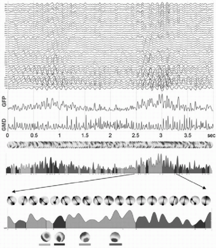 Figure 55.6 Microstate segmentation of spontaneous EEG. Four seconds of eyesclosed EEG measured from 42 electrodes are shown on top. The two blue curves represent the global field power (GFP) and the global map dissimilarity, respectively. A series of potential maps illustrate the data that has been submitted to a k-means cluster analysis with ignoring strength and polarity. Four maps best explained the whole 4 seconds of data. The four maps are illustrated on the bottom. On the GFP curve below the map series, the time periods during which each map was dominant are marked in different colors. A shorter period is zoomed in and all maps during this period are shown. Marking and connecting the extreme potentials illustrates the stability of topography during each period. (From Michel CM, Brandeis D. Data acquisition and pre-processing standards for electrical neuroimaging. In: Michel CM, Koenig T, Brandeis D, et al., eds. Electrical Neuroimaging. Cambridge, MA: Cambridge University Press; 2009.)(See color insert) |
EEG FORWARD PROBLEM
In this section, we introduce the methods for solving the so-called EEG forward problem, which deals with (i) how to model the neuronal excitation within the brain volume and (ii) how to model the head volume conduction process in order to quantitatively link neuronal electric sources with the electric potentials over the scalp. Solving the EEG forward problem can help understand the relationship between neuronal sources and the recorded EEG signals, and is also an integrative part of the EEG
inverse problem, which will be discussed in the section “EEG Inverse Problem.”
inverse problem, which will be discussed in the section “EEG Inverse Problem.”
Source Models
The primary sources of EEG are considered to be the postsynaptic currents flowing through the apical dendritic trees of cortical pyramidal cells. Such neuronal currents, when viewed from a location on the scalp surface that is relatively remote to where the neural excitation takes place (far field), can be modeled as an electric current dipole composed of a pair of current source and sink with infinitely small interdistance. When the brain electric activity is confined to a few focal regions, each of these focal areas of neuronal excitation may be modeled as an equivalent current dipole (ECD) based on the far field theory (for a theoretical treatment see the appendix in Chapter 5). Such equivalent dipole model has been widely used in source localization analysis of EEG in an attempt to better interpret the origins of the scalp-recorded EEG (116, 117, 118, 119 and 120). While the ECD is a simplified model and higher order equivalent source models such as the quadrupole have also been studied to represent the neural electric sources (121,122), the dipole model has been so far the most commonly used brain electric source model. A number of experimental and clinical studies have demonstrated its merits in helping interpreting EEG data and localizing sources generating the scalp-recorded EEG.
When the neuronal sources are no longer confined to a few focal regions, the ECD model may not well represent the distributed brain electric activity. Distributed current source models can then be used to represent the whole-brain bioelectric activity. The essence of the distributed current source models is to model the neuronal activities over a small region by a current dipole located at each region. The brain activity with any distribution of neuronal currents can be approximately represented by a source model consisting of a distribution of current dipoles that are evenly placed within the entire brain volume. At each location, three orthogonal dipoles are used in that the weighted combination of them is capable of representing an averaged current flow with an arbitrary direction in the region. Such source model is usually called volume current density (VCD) model, in which current dipoles distribute over the entire brain volume (123). The brain anatomical information can also be used to constrain the current source space to the cortical gray matter due to its dominant presence of large pyramidal cells. Such anatomical constraints can be obtained from existing structural neuroimaging modalities, particularly T1-weighted MRI, which provides high spatial resolution and a great contrast to differentiate the cortical gray matter from the white matter and cerebrospinal fluid (CSF). The current source orientations can be further constrained to be perpendicular to the cortical surface, because the columnar organization of neurons within the cortical gray matter constrains the regional current flow in either outward or inward normal direction with respect to the local cortical patch (124), and the gray matter thickness (about 2 to 4 mm) is much smaller relative to the “source-to-sensor” distance (60). Under such cortical constraints, such source model is usually called cortical current density (CCD) model, in which current dipoles distribute over a surface in parallel to the epicortical surface.
Related posts:

Stay updated, free articles. Join our Telegram channel

Full access? Get Clinical Tree


